Realized Volatility, Heterogeneous Market Hypothesis and the - PowerPoint PPT Presentation
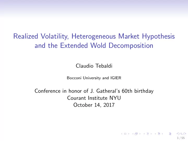
Realized Volatility, Heterogeneous Market Hypothesis and the Extended Wold Decomposition Claudio Tebaldi Bocconi University and IGIER Conference in honor of J. Gatherals 60th birthday Courant Institute NYU October 14, 2017 1 / 55 Foreword
Realized Volatility, Heterogeneous Market Hypothesis and the Extended Wold Decomposition Claudio Tebaldi Bocconi University and IGIER Conference in honor of J. Gatheral’s 60th birthday Courant Institute NYU October 14, 2017 1 / 55
Foreword on Impulse Response Functions ‘Dynamic economic models make predictions about impulse responses .....impulse responses quantify the exposure to long run macroeconomic shocks.... Financial markets provide compensations to investors who are exposed to these shocks.’ J. Borovicka L. Hansen 2016 This exotic research program came to my mind... World Bachelier Conference London 2008 Program - 08.30-09.30 Plenary lecture: Lars Peter Hansen ”Modelling the long run: valuation in dynamic stochastic economies” - 09.30-10.30 Plenary lecture: Jim Gatheral ”Consistent modelling of VIX and SPX options” JIM .... YOU’RE RESPONSIBILE! 2 / 55
Research Group on Impulse Response Functions • OTT with F. Ortu and A. Tamoni “Long Run Risk and the Persistence of Consumption Shocks ” The Review of Financial Studies (2013), 26 (11) 2876-2915. • BPTT with F.Bandi, B. Perron and A.Tamoni “The Scale of Predictability”, forthcoming Journal of Econometrics . • OSTT with F.Ortu, F. Severino and A.Tamoni “A persistence-based Wold-type decomposition for stationary time series”, Working Paper IGIER under review. • CVOST Cerreia-Vioglio, S., Ortu, F., Severino, F., Tebaldi, C., 2017. Multivariate Wold Decompositions. Working Paper IGIER n.606, Bocconi University • Rough Cascades and a potential resolution of Volatility and Interest Rate Puzzles. Daniele D’Ascenzo (now JP Morgan) Daniele D’Arienzo Bocconi PhD Candidate 3 / 55
Motivation of the Talk • Two well-established stylized facts that characterize economic fluctuations in dynamic economies and financial markets: - The ‘multiscale’ nature of information based agent decisions: intrinsic frequencies range from HFT trading decisions to secular trends. - Widespread observation of self-similarity and scale invariance. The ‘critical’ nature of economic fluctuations • Research Program: explore the implications of these facts on impulse response functions with particular attention to their normative rather than descriptive implications. • This talk: I will discuss the implications of these facts on log-volatility IRf to conclude that there are important ”structural” motivations that suggest the introduction of a Rough Cascade Volatility Model. 4 / 55
Plan of the talk • Impulse Response Functions in Dynamic Stochastic Economies. • Fluctuations Theory and Critical Phenomena: Scaling, Universality and Renormalization Group. • The Extended Wold Decomposition. • Heterogeneous Market Hypothesis, Resolution Filtration and Cascades of Shocks. • Volatility Forecasting with (Rough) Impulse Response Functions. 5 / 55
Literature on IRf • Slutsky (1927), Yule (1927) and Frisch (1933) formulated the concepts of “propagation” and “impulse” in economic time series. Wold (1938) formalizes the notion of IRF for a stationary time series. • Identification challenges in rational expectation models Sims (1980). • Hansen, Scheinkmann and Borovicka (2011-2016) introduce the modern non-linear continuous time extensions of IRf and its relation with Malliavin Derivatives and Option sensitivities. • Extension of the IRf as a relevant ’normative’ tool: see Boijnov Shepard (2017) ‘Time series experiments and causal estimands’. 6 / 55
Classical Wold Decomposition Given a zero-mean, regular, weakly stationary time series x = { x t } t ∈ Z , we have + ∞ ∑ x t = α h ε t − h + ν t ∀ t ∈ Z , h = 0 where the equality is in the L 2 -norm. • The process ε = { ε t } t ∈ Z is a unit variance white noise. • α h is the projection coefficient of x t on the linear space generated by the innovation ε t − h : α h = E [ x t ε t − h ] , h ∈ N 0 . α h is the impulse response function of x t to the shock ε t − h . • The deterministic component ν is orthogonal to ε , id est E [ ν t ε t − h ] = 0 ∀ h ∈ N 0 . 7 / 55
Fluctuations Theory and Critical Phenomena • (Widom) scaling law for Magnetization � � t = T − T c H M ( H , T ) = | t | β F | t | βδ T c where function F is a universal scaling such that: - M ∼ H 1 / δ for | t | = 0, - M ∼ | t | β for H = 0 and | t | → 0 • Kadanoff’s idea was that in the critical regime a thermodynamic system, due to the strong correlations among the microscopic variables, behaves as if constituted by rigid blocks of arbitrary size. • Wilson Renormalization group: a semigroup of transformations that produces a progressive elimination of the microscopic degrees of freedom to obtain the asymptotic large scale properties of the system. 8 / 55
Renormalization Group in a Nutshell • Renormalization Transformation and the Central Limit Theorem (Jona-Lasinio Phys. Reports 2001) Consider ξ 1 , ..., ξ n , .... i.i.d. with zero mean and unit variance, and define block variables: 2 n 2 n + 1 ξ i , then ζ n + 1 = ζ 1 n + ζ 2 n = 2 − n n = 2 − n ζ 1 ξ i , ζ 2 n ∑ ∑ √ 2 2 2 i = 1 i = 2 n + 1 and correspondingly on the densities: √ � � � ζ ζ ζ R p n : = dyp x 2 − y p n ( y ) n ζ ζ The fixed point of the transformation: R p ∞ = p ∞ selects the standard normal distribution. 9 / 55
Renormalization Group in a Nutshell II • The action of R in the vicinity of the fixed point: ζ ζ η 2 � � R p ∞ ( 1 + η h ) = p ∞ ( 1 + η L h ) + O defines a linear operator L : √ 2 � � � dye − y 2 h L h ( x ) : = √ π x 2 − y • Eigenfunctions are given by Hermite functions h n • Eigenvalues λ n = 2 1 − n 2 , 0 ≤ n < 2 relevant directions, n = 2 marginal, n > 2 irrelevant. 10 / 55
Renormalization Group in a Nutshell III • More generally the Renormalization Semigroup establishes a modified stochastic limiting procedure for stochastic correlated variables. E.g. Sinai defines an H − self similar process as a fixed point of a rescaling transformation: ζ n + 1 = ζ 1 n + ζ 2 2 H . n • Critical properties are determined by fixed points of proper RG procedures that connect microscopic model critical correlations to macroscopic observable behavior. • Information on eigenvalues and eigenfunctions of the linearized operator provide information on critical indices and on finite size scaling functions. 11 / 55
Rescaling Transformation on Time Series and Discrete Haar filter Multiresolution decomposition: J g ( j ) π ( J ) ∑ x t = + ˘ ∀ t ∈ Z . ˘ t t j = 1 π ( j ) is the average of size 2 j of past values of x t : • ˘ t 2 j − 1 = 1 π ( j ) ∑ ˘ x t − p . t 2 j p = 0 g ( j ) • ˘ is the difference between these averages: t g ( j ) π ( j − 1 ) π ( j ) = ˘ − ˘ t . ˘ t t 12 / 55
Rescaling Transformation and Persistence g ( j ) • Variables ˘ is associated with the level of persistence j : it captures t fluctuations of x t with half-life in [ 2 j − 1 , 2 j ) . In this way, disentangle low-frequency shocks from high-frequency fluctuations. • Decimation procedure is necessary to get rid of the spurious correlation due to the overlapping of observations in the construction g ( j ) of ˘ t . Decimation selects the relevant degrees of freedom removing redundant statistics. g ( j ) • Decimated (detail) components ˘ t − 2 j k are proportional to Haar Transform of the original time series and are in one-to-one relationship with the original time series. g ( j ) • However, even after decimation, variables ˘ may be correlated, not t useful to define an IRf. 13 / 55
Redundant vs Decimated observations ( a ) j • • • • • • • • • • ... ... π (2) π (2) π (2) π (2) π (2) π (2) π (2) π (2) 1 2 3 4 5 6 7 8 • ... • • • • • • • • • ... g (2) g (2) g (2) g (2) g (2) g (2) g (2) g (2) 1 2 3 4 5 6 7 8 • • • • • • • • • • ... g (1) g (1) g (1) g (1) g (1) g (1) g (1) g (1) ... 1 2 3 4 5 6 7 8 • • • • • • • • • • ... ... g 1 g 2 g 3 g 4 g 5 g 6 g 7 g 8 t Redundant decomposition ( b ) j • • • ... π (2) π (2) 4 8 • • • ... g (2) g (2) 4 8 • ... • • • • g (1) g (1) g (1) g (1) 2 4 6 8 • • • • • • • • • • ... ... g 1 g 2 g 3 g 4 g 5 g 6 g 7 g 8 t � �� � � �� � Block 1 Block 2 Decimated decomposition 14 / 55
The Abstract Wold Theorem A general approach to derive orthogonal decompositions of time series follows from the Abstract Wold Theorem, that involves an isometric operator on a Hilbert space. Theorem (Abstract Wold Theorem) Consider a Hilbert space H and an isometry V : H − → H , i.e. � V x , V y � = � x , y � ∀ x , y ∈ H . Then H decomposes into an orthogonal sum H = ˆ H ⊕ ˜ H , where + ∞ + ∞ ˆ � V j H , ˜ � V j L V H = H = j = 0 j = 0 and the wandering subspace L V is defined as L V = H ⊖ V H . 15 / 55
Recommend
More recommend
Explore More Topics
Stay informed with curated content and fresh updates.

