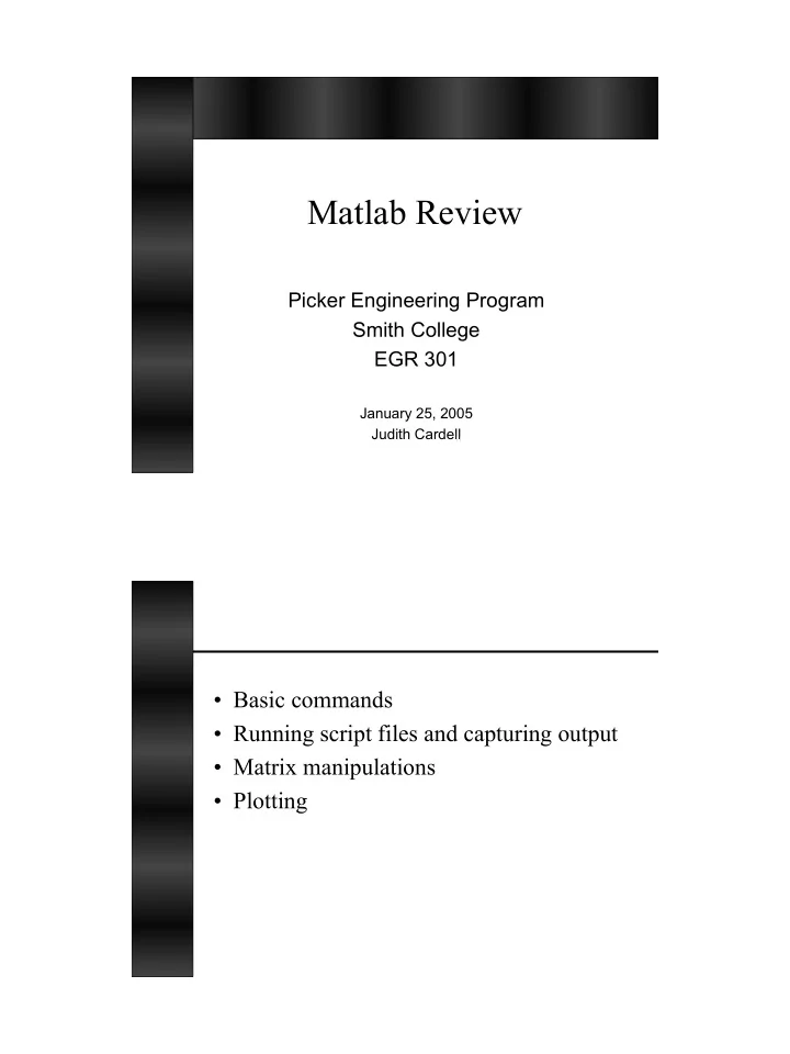
Matlab Review Picker Engineering Program Smith College EGR 301 - PDF document

Matlab Review Picker Engineering Program Smith College EGR 301 January 25, 2005 Judith Cardell • Basic commands • Running script files and capturing output • Matrix manipulations • Plotting

Matlab Hints • Matlab is available on the EGR, and most other, computers on campus • Icon: MATLAB 6.5.lnk Matlab Commands • pwd • ls • cd • edit • help command • See also webpage links and Appendix E of the EGR 220 text

Matlab Hints

Matlab Script File • Create a ‘.m’ file in the editor – Type “ edit filename ” in Matlab • Include comments!! – Header • Filename • Assignment and brief description • Your name and date – Comments throughout • ‘%’ is used to indicate a comment line • The semicolon tells Matlab not to echo the information on the given line to the screen Node-voltage equations by inspection • Find i 1 , i 2 , i 3 and i (problem 3.41)

Analysis by Inspection Ohm’s law V = IR � RI = V – R kk = sum of R in mesh k – R jk = negative sum of R in common between meshes j and k % % MatlabSample1.m % Your name, date ... % % Problem number 3.41 R = [ 12 -2 0 -2 7 -1 0 -1 6]; % The ; tells Matlab ... V = [6 -8 2]'; % Note the ' % % Our equation is R I = V % Solve for I by solving I = inverse(R) V % I = inv(R)*V % There is no ; here i = I(3) - I(2)

Running MatlabSample1.m • Run your script (.m) file in Matlab –Once it does what you want, record your results • To record your results, type diary filename .txt name-of-.m-file (note, the output will scroll across the screen when you run your script. The name-of- .m-file in this example is MatlabSample1 ) diary off >> diary Sample1Out.txt >> MatlabSample1 I = 0.3291 -1.0256 0.1624 i = 1.1880 >> diary off

EDIT Your Diary File!!!! Problem 3.41, output from MatlabSample1.m I = % Current vector, i1, i2 and i3 0.3291 -1.0256 0.1624 i = % Current through 1 Ω resistor 1.1880 General Matrix Manipulations • Matrix – An m x n collection of data – (rows x columns) • Vector – An m x 1 array, or – A 1 x n array • Matrix manipulation in Matlab – The ‘:’ operator to select rows, columns or subsets of rows and columns

>> A = [ 1 2 3 4 ; 5 6 7 8 ; 3 4 5 6 ; 2 6 4 5] A = 1 2 3 4 5 6 7 8 3 4 5 6 2 6 4 5 >> B = [A(1,:)] B = 1 2 3 4 >> C = [A(:,2)] C = 2 6 4 6 >> D = [A(1:2,2)] D = 2 6 >> A = [ 1 2 3 4 ; 5 6 7 8 ; 3 4 5 6 ; 2 6 4 5] A = 1 2 3 4 5 6 7 8 3 4 5 6 2 6 4 5 >> F = [A(1,:) A(3,:)] F = 1 2 3 4 3 4 5 6 >> G = [A(1,:) ; A(3,:)] G = 1 2 3 4 3 4 5 6

Matrix Multiplication • Standard matrix multiplication – A * B • Element-wise multiplication – Do Not mistake this for matrix multiplication – A .* B >> A = [ 1 1 ; 1 1; 1 1] A = 1 1 1 1 1 1 >> B = A‘ ( Matrix transpose ) B = 1 1 1 1 1 1 >> C = B * A C = 3 3 3 3 >> D = B .* A ??? Error using ==> .* Matrix dimensions must agree. >> D = B(:,1:2) .* A(1:2,:) D = 1 1 1 1

Plotting • 2-D plots – Input or create x- and y- axis data sets – plot (x, y, ‘b--’) – Also contour() , based on x, y, z data • 3-D plots – Input or create x-, y- and z- axis data sets – mesh (x, y, z) – Or, setup x- and y-axes with meshgrid() – Also: surf()

Plotting • Scale axes with axis() command • To create time step data for x-axis t = [start-value: step-size: end-value] >> t = [0:0.5:5] t = 0.0 0.5 1.0 1.5 2.0 2.5 3.0 3.5 4.0 4.5 5.0 • Label axes and plots – title(), xlabel(), ylabel() • For plotting more than one line ‘ hold on’ and ‘hold off’ can be useful