Math 211 Math 211 Lecture #28 December 7, 2000 2 Predator-Prey - PDF document
1 Math 211 Math 211 Lecture #28 December 7, 2000 2 Predator-Prey Predator-Prey Lotka-Volterra system x = ( a by ) x (prey fish) y = ( c + dx ) y (predator sharks) Equilbrium points (0 , 0) is a saddle. (
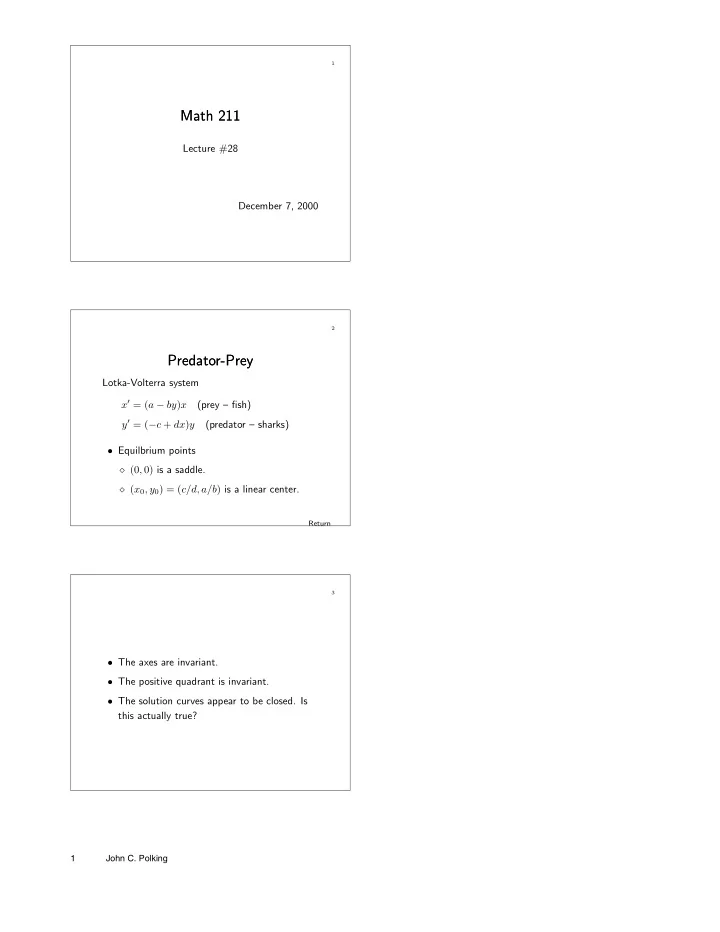
1 Math 211 Math 211 Lecture #28 December 7, 2000 2 Predator-Prey Predator-Prey Lotka-Volterra system x ′ = ( a − by ) x (prey – fish) y ′ = ( − c + dx ) y (predator – sharks) • Equilbrium points ⋄ (0 , 0) is a saddle. ⋄ ( x 0 , y 0 ) = ( c/d, a/b ) is a linear center. Return 3 • The axes are invariant. • The positive quadrant is invariant. • The solution curves appear to be closed. Is this actually true? 1 John C. Polking
4 Along the solution curve y = y ( x ) we have dy dx = y ( − c + dx ) x ( a − by ) . The solution is H ( x, y ) = by − a ln y + dx − c ln x = C • This is an implicit equation for the solution curve. ⇒ All solution curves are closed, and represent periodic solutions. System Return 5 Why Fishing Leads to More Fish Why Fishing Leads to More Fish Compute the average of the fish & shark populations. dt ln x ( t ) = x ′ d x = a − by � T 0 = 1 d dt ln x ( t ) dt = a − by. T 0 So y = a/b = y 0 . Similarly x = x 0 = c/d. System Return 6 The effect of fishing that does not distinquish between fish and sharks is the system x ′ = ( a − by ) x − ex y ′ = ( − c + dx ) y − ey This is the same system with a replaced by a − e and c replaced by c + e . System Averages 2 John C. Polking
7 The average populations are x 1 = c + e y 1 = a − e and d b Fishing causes the average fish population to increase and the average shark population to decrease. Averages 8 Cottony Cushion Scale Insect & Cottony Cushion Scale Insect & the Ladybird Beetle the Ladybird Beetle • Cottony cushion scale insect accidentally introduced from Australia in 1868. ⋄ Threatened the citrus industry. • Ladybird beetle imported from Australia ⋄ Natural predator – reduced the insects to manageable low. Return 9 DDT kills the scale insect. • Massive spraying ordered. ⋄ Despite the warnings of mathematicians and biologists. • The scale insect increased in numbers, as predicted by Volterra. 3 John C. Polking
10 Model of the Immune System in Model of the Immune System in Action Action • How does the immune system develops immunity to virus caused diseases? ⋄ Diseases such as flu, the cold, mumps, . . . • Infectious Diseases of Humans - Roy M. Anderson & Robert M. May, Oxford University Press 1992 11 The model includes the interactions between virus cells and lymphocytes generated by the immune system. • V ( t ) = number of virus cells • Two types of lymphocytes, E 1 ( t ) & E 2 ( t ) . 12 Lymphocytes Lymphocytes Both types: • Are recruited from bone marrow at a constant rate • Die at a rate proportional to their numbers • Proliferate due to contact with each other Return 4 John C. Polking
13 Model With No Virus Present Model With No Virus Present E 1 E 2 E ′ 1 = Λ 1 − µ 1 E 1 + a 1 1 + b 1 E 1 E 2 E 1 E 2 E ′ 2 = Λ 2 − µ 2 E 2 + a 2 1 + b 2 E 1 E 2 • For pplane5 use parameters Λ 1 = Λ 1 = 1 , µ 1 = µ 1 = 1 . 25 , a 1 = a 2 = 0 . 252 , and b 1 = b 2 = 0 . 008 . E cells Return 14 Dynamics of the Lymphocytes Dynamics of the Lymphocytes E 1 ’ = 1 − 1.25 E 1 + 0.252 E 1 E 2 /(1 + 0.008 E 1 E 2 ) E 2 ’ = 1 − 1.25 E 2 + 0.252 E 1 E 2 /(1 + 0.008 E 1 E 2 ) 30 25 Immune State 20 E 2 15 10 5 Virgin State 0 0 5 10 15 20 25 30 E 1 Return 15 Interactions with the Virus Interactions with the Virus • Virus cells have an intrinsic growth rate r. • Lymphocytes of type E 1 : ⋄ kill virus because of contacts with them ⋄ proliferate because of contacts with virus • Lymphocytes of type E 2 : ⋄ do not directly interact with the virus ⋄ regulate cells of type E 1 Return 5 John C. Polking
16 Model With Virus Present Model With Virus Present E 1 E 2 E ′ 1 = Λ 1 − µ 1 E 1 + a 1 + KV E 1 1 + b 1 E 1 E 2 E 1 E 2 E ′ 2 = Λ 2 − µ 2 E 2 + a 2 1 + b 2 E 1 E 2 V ′ = rV − kV E 1 • For ode45 use K = 0 . 5 , k = 0 . 01 and r = 0 . 1 . No virus Interactions Return 17 Equilibrium Points Equilibrium Points • There are three realistic equilibrium points E 1 1 5 20 = , , E 2 1 5 & 20 V 0 0 0 • The first two are unstable. The third is asymptotically stable. • What is the global behavior? The best we can do is to check with ode45 . System Dynamics No virus 6 John C. Polking
Recommend
More recommend
Explore More Topics
Stay informed with curated content and fresh updates.
