
SLIDE 1
Marching Cubes
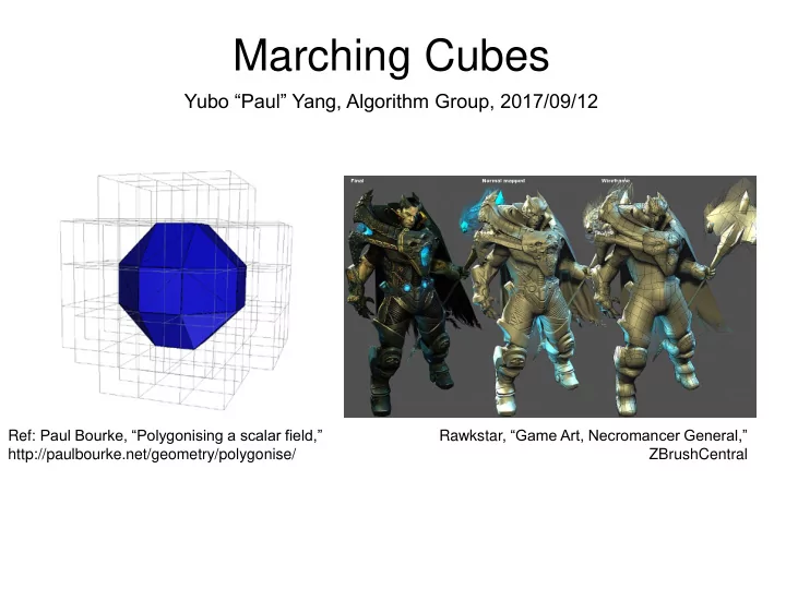
Yubo “Paul” Yang, Algorithm Group, 2017/09/12
Ref: Paul Bourke, “Polygonising a scalar field,” http://paulbourke.net/geometry/polygonise/ Rawkstar, “Game Art, Necromancer General,” ZBrushCentral
Marching Cubes Yubo Paul Yang, Algorithm Group, 2017/09/12 Ref : - - PowerPoint PPT Presentation
Marching Cubes Yubo Paul Yang, Algorithm Group, 2017/09/12 Ref : Paul Bourke, Polygonising a scalar field, Rawkstar , Game Art, Necromancer General, http://paulbourke.net/geometry/polygonise/ ZBrushCentral Showcase I: s,p,d
Yubo “Paul” Yang, Algorithm Group, 2017/09/12
Ref: Paul Bourke, “Polygonising a scalar field,” http://paulbourke.net/geometry/polygonise/ Rawkstar, “Game Art, Necromancer General,” ZBrushCentral
Ref: Paul Bourke, “Polygonising a scalar field,” http://paulbourke.net/geometry/polygonise/
Find N-1 representation of the zero-crossings of an N dimensional scalar field 𝑔 𝑦 = 0. To simplify discussion:
Ref: Paul Bourke, “Polygonising a scalar field,” http://paulbourke.net/geometry/polygonise/
Form a facet approximation for an isosurface of a scalar field sampled
Triangle 1 Triangle 2 Triangle 3 Triangle 8 … 3x3x3 samples of 𝒇−𝒔𝟑
Ref: Paul Bourke, “Polygonising a scalar field,” http://paulbourke.net/geometry/polygonise/
This is what a Gaussian looks like!
by Paul Bourke Ref: “Polygonising a scalar field”, http://paulbourke.net/geometry/polygonise/
by Paul Bourke Ref: “Polygonising a scalar field”, http://paulbourke.net/geometry/polygonise/ 1 7 6 5 4 3 2 1 vertex < iso. 1 1 1 11 10 9 8 7 6 5 4 3 2 1 edge intersect Edge table
by Paul Bourke Ref: “Polygonising a scalar field”, http://paulbourke.net/geometry/polygonise/ (𝑄
1, 𝑊 1)
𝑄
1 + 𝑊 𝑗𝑡𝑝 − 𝑊 1
2 − 𝑊 1
(𝑄
2, 𝑊 2)
𝑊
𝑗𝑡𝑝
Linear Interpolation:
by Paul Bourke Ref: “Polygonising a scalar field”, http://paulbourke.net/geometry/polygonise/
Triangle list = [ (3,11,2) ] 𝑄3 = [ intersect at edge 3] 𝑄
11 = [ intersect at edge 11]
𝑄2 = [ intersect at edge 2]
11
by Paul Bourke Ref: “Polygonising a scalar field”, http://paulbourke.net/geometry/polygonise/ 1 1 7 6 5 4 3 2 1 vertex < iso. 11 10 9 8 7 6 5 4 3 2 1 edge intersect Edge table 1 1 1 1
consider.
Wikipedia
The marching cubes algorithm is almost entirely table look-up Slowness in matplotlib is likely due to 2D projection overhead (matplotlib does not do actual 3D rendering) Timing of skimage.measure.marching_cubes_lewiner
Dot averaged face normal vectors with light rays to determine luminescence
Mikola Lysenko, “Smooth Voxel Terrain” (2012) S.F. Gibson, (1999) “Constrained Elastic Surface Nets” Mitsubishi Electric Research Labs, Technical Report.
Compute the edge crossings (like we did in marching cubes) and then take their center of mass as the vertex for each cube. Fewer vertices than marching cubes
[1] Paul Bourke, “Polygonising a scalar field” (1994) [2] Mikola Lysenko, “Smooth Voxel Terrain” (2012) [3] Sarah F. Gibson, “Constrained Elastic Surface Nets” (1999)