Management Strategies and Dynamic Financial Analysis Dynamic - PowerPoint PPT Presentation
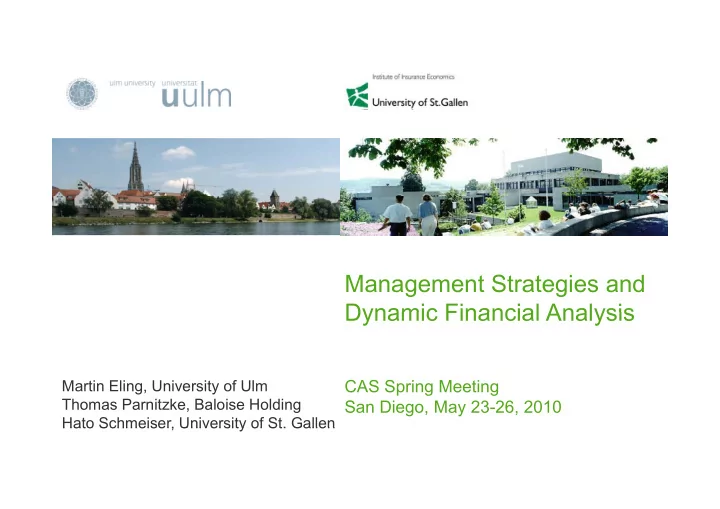
Management Strategies and Dynamic Financial Analysis Dynamic Financial Analysis CAS Spring Meeting Martin Eling, University of Ulm Thomas Parnitzke, Baloise Holding San Diego, May 23-26, 2010 Hato Schmeiser, University of St. Gallen Hato
Management Strategies and Dynamic Financial Analysis Dynamic Financial Analysis CAS Spring Meeting Martin Eling, University of Ulm Thomas Parnitzke, Baloise Holding San Diego, May 23-26, 2010 Hato Schmeiser, University of St. Gallen Hato Schmeiser, University of St. Gallen
Eling, Parnitzke, Schmeiser| Management Strategies and Dynamic Financial Analysis Page 2 Outline 1. Motivation 2. Model Framework 3. Management Strategies 4. Performance Measurement 5 5. Simulation Study Si l ti St d 6. Role of Non-linear Dependencies 7. Conclusion and Outlook
Eling, Parnitzke, Schmeiser| Management Strategies and Dynamic Financial Analysis Page 3 1. Motivation: Three pillars of Solvency II Solvency II Solvency II First pillar: Second pillar: Third pillar: Quantitative regulations for Qualitative elements of Market transparency and capital requirements supervision disclosure requirements → Technical provisions, → Technical provisions → Appropriate processes → Appropriate processes → A transparent process will → A transparent process will minimum capital, and decisions in the context require less regulation as target capital of a risk management market participants → Use of standard models system themselves force appropriate and internal models → Principles for internal risk insurer behavior (Dynamic Financial management and control → Harmonization with IFRS Analysis)
Eling, Parnitzke, Schmeiser| Management Strategies and Dynamic Financial Analysis Page 4 1. Motivation: Dynamic Financial Analysis (DFA) • Projects results under a variety of possible scenarios, showing how outcomes might be affected by changing internal and external conditions g y g g • Used in practice for Insurance Assets Liabilities Company cash flow projection and decision support Risk Management Environ- Capital Regulation Competition ment Market • Aim of this paper: Ai f thi 1. Implement management strategies in a DFA framework 2 Study the effects on the insurer’s risk and return position 2. Study the effects on the insurer s risk and return position 3. Give helpful insights for the development of DFA tools
Eling, Parnitzke, Schmeiser| Management Strategies and Dynamic Financial Analysis Page 5 2. Model Framework • Simplified model of a property-liability insurer Assets Assets Liabilities Liabilities • Balance sheet (t=0): Investments Equity (stocks, bonds, Reserves etc.) (Premiums) Investment Underwriting g Result Result • Statement of Income (t=1): Premiums - Claims Claims - Costs (Upfront, Claim Settlement) = Underwriting Result + Investment Result = Earnings Earnings
Eling, Parnitzke, Schmeiser| Management Strategies and Dynamic Financial Analysis Page 6 2. Model Framework: Earnings (1) EC EC E Insurance Assets Liabilities 1 Company t t t Risk Management (2) (2) max( max( ( ( ) 0) ),0) E E I I U U tr tr I I U U t t t t t Environ- Capital Regulation ment Competition Market EC : Equity Capital at the end of period t t E E : Earnings E i t I : Investment Result t U : Underwriting Result t tr : Tax rate
Eling, Parnitzke, Schmeiser| Management Strategies and Dynamic Financial Analysis Page 7 2. Model Framework: Investment result P (3) I r ( EC P Ex ) Insurance Assets Liabilities t pt t 1 t 1 t 1 Company Risk Management (4) (4) r r 1 1 r pt t 1 1 t t 1 2 t Environ- Capital Regulation ment Competition Market r : Return of investment portfolio pt P : Premiums t t 1 P Ex : Upfront costs (depending on premiums) t 1 : Portion invested in high-risk investments t 1 r 1 : Return of high-risk investment (e.g., stocks : Ret rn of high risk in estment (e g stocks ) ) t r : Return of low-risk investment (e.g., bonds) 2 t
Eling, Parnitzke, Schmeiser| Management Strategies and Dynamic Financial Analysis Page 8 2. Model Framework: Underwriting result P C (5) U P C Ex Ex Insurance Assets Liabilities t t 1 t t 1 t Company Risk Management EC EC (6) (6) P P cr MV MV t t 1 1 t 1 t 1 t 1 t 1 Environ- Capital Regulation ment Competition Market • Consumer response (cr) to changes in solvency cr 1, if EC MCR t cr 1, 1 if EC if EC MCR MCR t • Underwriting cycle ( π ): Markov chain with different states C Ex : Claim settlement costs t • Claims: C C C : Consumer response cr t cat ncat t t t : Underwriting cycle : Underwriting cycle MCR : Minimum capital required (Solvency I) : Portion in the underwriting market t 1
Eling, Parnitzke, Schmeiser| Management Strategies and Dynamic Financial Analysis Page 9 2. Model: Implementation in R (simplified one period example) E=0 # Liabilities EC=15 mu=log(0.85)-0.5*log(1+0.085^2/0.85^2) MV=200 MV 200 sigma= (log(1+0.085^2/0.85^2))^(1/2) i (l (1 0 085^2/0 85^2))^(1/2) β =0.2 C<-rlnorm(1,mu,sigma)*P P=MV* β ExC<-0.05*C ExP<-0.05*P U<-P-C-ExP-ExC tr=0.25 # Aggregation α =0 2 α =0.2 E[i]< I+U max(tr*(I+U) 0) E[i]<-I+U-max(tr (I+U),0) } #end for i for (i in 1:10000) { hist (E) # Assets mean(E) rp<- α *rnorm(1,0.1,0.2)+ sd(E) (1- α )*rnorm(1,0.05,0.05) (1 α ) rnorm(1,0.05,0.05) summary(E) I<-rp*(EC+P-ExP)
Eling, Parnitzke, Schmeiser| Management Strategies and Dynamic Financial Analysis Page 10 3. Management Strategies Insurance Assets Liabilities • At the beginning of each period Company Risk management can change: management can change: Management - Portion of the risky investment ( α ) Environ- Capital Regulation ment Competition Market - Share in the underwriting business ( β ) g ( β ) • Three Strategies under consideration: Strategy St t S l Solvency Hi h Ri k High Risk G Growth th Risk Reduction and Target Risk Reduction Risk Taking Risk Taking EC t < EC t > Trigger EC t < MCR t ·1.5 EC t < MCR t ·1.5 MCR t ·1.5 MCR t ·1.5 α and β d β α and β d β α and β d β β β Rule 0.05 ↓ 0.05 ↑ 0.05 ↓ 0.05 ↑
Eling, Parnitzke, Schmeiser| Management Strategies and Dynamic Financial Analysis Page 11 4. Performance Measurement Symbol Measure Interpretation Return E(G) Expected gain per annum Absolute return ROI Expected return on investment per annum p p Relative return Risk σ (G) Standard deviation of gain per annum Total risk RP Ruin probability p y Downside risk EPD Expected policyholder deficit Downside risk Perfor- SR σ Sharpe ratio Return/total risk mance mance SR RP Modified Sharpe ratio (RP) Return/downside risk SR SR EPD Modified Sharpe ratio (EPD) Modified Sharpe ratio (EPD) Return/downside risk Return/downside risk
Eling, Parnitzke, Schmeiser| Management Strategies and Dynamic Financial Analysis Page 12 5. Simulation Study: Model Specifications • Time horizon: T = 5 years, equity capital in t = 0: €15 million • Trigger for the management strategies: Solvency I MCR·1.5 gg g g y • Investments ( α ): High-risk N (0.1,0.2), low-risk N (0.05,0.05) • Underwriting business ( β ): Market volume €200 million - Log-normally distributed claims LN (0.85,0.085) - Underwriting cycle with three different states 0.3 0.5 0.2 (1.05, 1, 0.95) and the transition probabilities p 0.2 0.6 0.2 sj 0.1 0.5 0.4 - Consumer response: 0.95 if EC < MCR·1.5 • Tax rate: 25% Assets Liabilities Insurance Company Risk Management Management Environ- Capital Regulation ment Competition Market
Eling, Parnitzke, Schmeiser| Management Strategies and Dynamic Financial Analysis Page 13 5. Simulation Study: Results Strategy No Strategy Solvency High Risk Growth Return E(G) in million € 5.57 5.46 5.70 7.30 ROI in % 23.35 23.05 23.73 27.99 Risk σ (G) in million € 2.88 2.95 2.89 4.19 RP in % 0.22 0.06 0.63 0.20 EPD in million € 0.0045 0.0006 0.0225 0.0035 Perfor- SR σ 1.93 1.85 1.97 1.74 mance mance SR RP 12.42 48.75 4.50 18.52 SR EPD 6.18 43.48 1.26 10.49
Eling, Parnitzke, Schmeiser| Management Strategies and Dynamic Financial Analysis Page 14 5. Simulation Study: Robustness Checks / Sensitivity Analysis • Variation of the equity capital in t=0 (from €10 to €20 million) • Variation of the time horizon (from 1 to 10 years) ( y ) • Variation of starting values (application of different α and β in t=0) • Variation of the step length (for changes induced by the management, different step lengths for α and β are assumed) • Variation of consumer response function
Eling, Parnitzke, Schmeiser| Management Strategies and Dynamic Financial Analysis Page 15 5. Simulation Study: Variation of the equity capital in t=0 per annum No Strategy Solvency Limited Growth 8 7 xpected gain p 6 5 ex 4 10 11 12 13 14 15 16 17 18 19 20 equity capital in t = 0 4% No Strategy Solvency Limited Growth in probability 3% 2% rui 1% 0% 10 10 11 11 12 12 13 13 14 14 15 15 16 16 17 17 18 18 19 19 20 20 equity capital in t = 0
Recommend
More recommend
Explore More Topics
Stay informed with curated content and fresh updates.
![COMMUNICATING [with empathy] @ DY DYNAMIC JILL JILL @ DY DYNAMIC JILL TENSION IS INEVITABLE @](https://c.sambuz.com/548934/communicating-s.webp)
