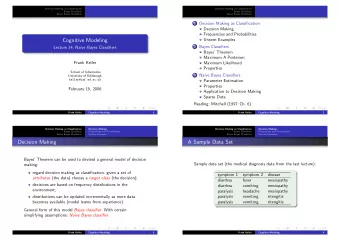
Machine Learning and Data Mining 2 : Bayes Classifiers Kalev Kask - PowerPoint PPT Presentation

+ Machine Learning and Data Mining 2 : Bayes Classifiers Kalev Kask

A basic classifier • Training data D={x (i) ,y (i) }, Classifier f(x ; D) – Discrete feature vector x – f(x ; D) is a contingency table • Ex: credit rating prediction (bad/good) – X 1 = income (low/med/high) – How can we make the most # of correct predictions? Features # bad # good X=0 42 15 X=1 338 287 X=2 3 5 (c) Alexander Ihler 2

A basic classifier • Training data D={x (i) ,y (i) }, Classifier f(x ; D) – Discrete feature vector x – f(x ; D) is a contingency table • Ex: credit rating prediction (bad/good) – X 1 = income (low/med/high) – How can we make the most # of correct predictions? – Predict more likely outcome for each possible observation Features # bad # good X=0 42 15 X=1 338 287 X=2 3 5 (c) Alexander Ihler 3

A basic classifier • Training data D={x (i) ,y (i) }, Classifier f(x ; D) – Discrete feature vector x – f(x ; D) is a contingency table • Ex: credit rating prediction (bad/good) – X 1 = income (low/med/high) – How can we make the most # of correct predictions? – Predict more likely outcome for each possible observation Features # bad # good – Can normalize into probability: X=0 .7368 .2632 p( y=good | X=c ) X=1 .5408 .4592 X=2 .3750 .6250 – How to generalize? (c) Alexander Ihler 4

Bayes Rule • Two events: headache, flu • p(H) = 1/10 • p(F) = 1/40 H • p(H|F) = 1/2 F • You wake up with a headache – what is the chance that you have the flu? Example from Andrew Moore ’ s slides

Bayes Rule • Two events: headache, flu • p(H) = 1/10 • p(F) = 1/40 H • p(H|F) = 1/2 F • P(H & F) = ? • P(F|H) = ? Example from Andrew Moore ’ s slides

Bayes rule • Two events: headache, flu • p(H) = 1/10 • p(F) = 1/40 H • p(H|F) = 1/2 F • P(H & F) = p(F) p(H|F) = (1/2) * (1/40) = 1/80 • P(F|H) = ? Example from Andrew Moore ’ s slides

Bayes rule • Two events: headache, flu • p(H) = 1/10 • p(F) = 1/40 H • p(H|F) = 1/2 F • P(H & F) = p(F) p(H|F) = (1/2) * (1/40) = 1/80 • P(F|H) = p(H & F) / p(H) = (1/80) / (1/10) = 1/8 Example from Andrew Moore ’ s slides

Classification and probability • Suppose we want to model the data • Prior probability of each class, p(y) – E.g., fraction of applicants that have good credit • Distribution of features given the class, p(x | y=c) – How likely are we to see “ x ” in users with good credit? • Joint distribution • Bayes Rule: (Use the rule of total probability to calculate the denominator!) (c) Alexander Ihler

Bayes classifiers • Learn “ class conditional ” models – Estimate a probability model for each class • Training data – Split by class – D c = { x (j) : y (j) = c } • Estimate p(x | y=c) using D c • For a discrete x, this recalculates the same table… Features # bad # good p(x | p(x | p(y=0|x) p(y=1|x) y=0) y=1) X=0 42 15 .7368 .2632 42 / 15 / 307 X=1 338 287 .5408 .4592 383 X=2 3 5 .3750 .6250 338 / 383 287 / 307 3 / 383 5 / 307 p(y) 383/690 307/690 (c) Alexander Ihler

Bayes classifiers • Learn “ class conditional ” models – Estimate a probability model for each class • Training data – Split by class – D c = { x (j) : y (j) = c } • Estimate p(x | y=c) using D c • For continuous x, can use any density estimate we like – Histogram – Gaussian 12 – … 10 8 6 4 2 0 -3 -2 -1 0 1 2 3 (c) Alexander Ihler

Gaussian models • Estimate parameters of the Gaussians from the data Feature x 1 ! (c) Alexander Ihler

Multivariate Gaussian models • Similar to univariate case ¹ = length-d column vector § = d x d matrix | § | = matrix determinant 5 Maximum likelihood estimate: 4 3 2 1 0 -1 -2 -2 -1 0 1 2 3 4 5 (c) Alexander Ihler

Example: Gaussian Bayes for Iris Data • Fit Gaussian distribution to each class {0,1,2} (c) Alexander Ihler 14

Bayes classifiers • Estimate p(y) = [ p(y=0) , p(y=1) …] • Estimate p(x | y=c) for each class c • Calculate p(y=c | x) using Bayes rule • Choose the most likely class c • For a discrete x, can represent as a contingency table… – What about if we have more discrete features? Features # bad # good p(x | p(x | p(y=0|x) p(y=1|x) y=0) y=1) X=0 42 15 .7368 .2632 42 / 15 / 307 X=1 338 287 .5408 .4592 383 X=2 3 5 .3750 .6250 338 / 383 287 / 307 3 / 383 5 / 307 p(y) 383/690 307/690 (c) Alexander Ihler

Joint distributions • Make a truth table of all A B C 0 0 0 combinations of values 0 0 1 0 1 0 0 1 1 1 0 0 1 0 1 1 1 0 1 1 1 (c) Alexander Ihler

Joint distributions • Make a truth table of all A B C p(A,B,C | y=1) 0 0 0 0.50 combinations of values 0 0 1 0.05 0 1 0 0.01 • For each combination of values, 0 1 1 0.10 1 0 0 0.04 determine how probable it is 1 0 1 0.15 1 1 0 0.05 1 1 1 0.10 • Total probability must sum to one • How many values did we specify? (c) Alexander Ihler

Overfitting & density estimation • Estimate probabilities from the data A B C p(A,B,C | y=1) – E.g., how many times (what fraction) 0 0 0 4/10 0 0 1 1/10 did each outcome occur? 0 1 0 0/10 0 1 1 0/10 • M data << 2^N parameters? 1 0 0 1/10 1 0 1 2/10 1 1 0 1/10 • What about the zeros? 1 1 1 1/10 – We learn that certain combinations are impossible? – What if we see these later in test data? • Overfitting! (c) Alexander Ihler

Overfitting & density estimation A B C p(A,B,C | y=1) • Estimate probabilities from the data 0 0 0 4/10 – E.g., how many times (what fraction) 0 0 1 1/10 did each outcome occur? 0 1 0 0/10 0 1 1 0/10 • M data << 2^N parameters? 1 0 0 1/10 1 0 1 2/10 1 1 0 1/10 • What about the zeros? 1 1 1 1/10 – We learn that certain combinations are impossible? – What if we see these later in test data? • One option: regularize • Normalize to make sure values sum to one… (c) Alexander Ihler

Overfitting & density estimation • Another option: reduce the model complexity – E.g., assume that features are independent of one another • Independence: • p(a,b) = p(a) p(b) • p( x 1 , x 2 , … x N | y=1) = p( x 1 | y=1) p( x 2 | y=1) … p( x N | y=1) • Only need to estimate each individually A B C p(A,B,C | y=1) 0 0 0 .4 * .7 * .1 0 0 1 .4 * .7 * .9 0 1 0 .4 * .3 * .1 A p(A B p(B |y=1) C p(C |y=1) 0 1 1 … |y=1) 0 .7 0 .1 1 0 0 0 .4 1 .3 1 .9 1 0 1 1 .6 1 1 0 1 1 1 (c) Alexander Ihler

Example: Naïve Bayes Observed Data: x 1 x 2 y 1 1 0 1 0 0 1 0 1 0 0 0 0 1 1 1 1 0 0 0 1 1 0 1 Prediction given some observation x? < > Decide class 0 (c) Alexander Ihler 22

Example: Naïve Bayes Observed Data: x 1 x 2 y 1 1 0 1 0 0 1 0 1 0 0 0 0 1 1 1 1 0 0 0 1 1 0 1 (c) Alexander Ihler 23

Example: Joint Bayes Observed Data: x 1 x 2 y 1 1 0 1 0 0 1 0 1 x 1 x 2 p(x | y=0) x 1 x 2 p(x | y=1) 0 0 0 0 0 1/4 0 0 1/4 0 1 1 0 1 0/4 0 1 1/4 1 1 0 1 0 1/4 1 0 2/4 0 0 1 1 1 2/4 1 1 0/4 1 0 1 (c) Alexander Ihler 24

Naïve Bayes Models • Variable y to predict, e.g. “auto accident in next year?” • We have *many* co-observed vars x =[x 1 … x n ] – Age, income, education, zip code, … • Want to learn p(y | x 1 … x n ), to predict y – Arbitrary distribution: O(d n ) values! • Naïve Bayes: – p(y| x )= p( x |y) p(y) / p( x ) ; p( x |y) =  i p(x i |y) – Covariates are independent given “ cause ” • Note: may not be a good model of the data – Doesn’ t capture correlations in x ’ s – Can’ t capture some dependencies • But in practice it often does quite well! (c) Alexander Ihler

Naïve Bayes Models for Spam • y 2 {spam, not spam} • X = observed words in email – Ex: [ “ the ” … “ probabilistic ” … “ lottery ” …] – “ 1 ” if word appears; “ 0 ” if not • 1000’ s of possible words: 2 1000s parameters? • # of atoms in the universe: » 2 270 … • Model words given email type as independent • Some words more likely for spam ( “ lottery ” ) • Some more likely for real ( “ probabilistic ” ) • Only 1000’s of parameters now… (c) Alexander Ihler

Naïve Bayes Gaussian Models ¾ 2 11 0 x 2 0 ¾ 2 22 Again, reduces the number of parameters of the model: Bayes: n 2 /2 Naïve Bayes: n ¾ 2 11 > ¾ 2 x 1 22 (c) Alexander Ihler

You should know … • Bayes rule; p(y | x) = p(x|y)p(y)/p(x) • Bayes classifiers – Learn p( x | y=C ) , p( y=C ) • Maximum likelihood (empirical) estimators for – Discrete variables – Gaussian variables – Overfitting; simplifying assumptions or regularization • Naïve Bayes classifiers – Assume features are independent given class: p( x | y=C ) = p( x 1 | y=C ) p( x 2 | y=C ) … (c) Alexander Ihler

A Bayes Classifier • Given training data, compute p( y=c| x) and choose largest • What’s the (training) error rate of this method? Features # bad # good X=0 42 15 X=1 338 287 X=2 3 5 (c) Alexander Ihler 30