Evaluation Measures Sebastian Plsterl Computer Aided Medical - PowerPoint PPT Presentation
Evaluation Measures Sebastian Plsterl Computer Aided Medical Procedures | Technische Universitt Mnchen April 28, 2015 Outline 1 Classification 1. Confusion Matrix 2. Receiver operating characteristics 3. Precision-Recall Curve 2
Evaluation Measures Sebastian Pölsterl Computer Aided Medical Procedures | Technische Universität München April 28, 2015
Outline 1 Classification 1. Confusion Matrix 2. Receiver operating characteristics 3. Precision-Recall Curve 2 Regression 3 Unsupervised Methods 4 Validation 1. Cross-Validation 2. Leave-one-out Cross-Validation 3. Bootstrap Validation 5 How to Do Cross-Validation Sebastian Pölsterl 2 of 49
Performance Measures: Classification Confusion Matrix Deterministic Scoring Classifiers Classifiers Graphical Summary Multi-class Single-class Measures Statistics TP/FP Rate, Precision, Recall, ROC Curves Area under the No Change Change Sensitivity, PR Curves curve Correction Correction Specificity, Lift Charts H Measure F 1 -Measure, Dice , Cost Curves Geometric Mean Accuracy Error Rate Chohen’s Kappa Micro/Macro Fleiss’ Kappa Average Sebastian Pölsterl 3 of 49
Test Outcomes Let us consider a binary classification problem: • True Positive (TP) = positive sample correctly classified as belonging to the positive class • False Positive (FP) = negative sample misclassified as belonging to the positive class • True Negative (TN) = negative sample correctly classified as belonging to the negative class • False Negative (FN) = positive sample misclassified as belonging to the negative class Sebastian Pölsterl 4 of 49
Confusion Matrix I Ground Truth Class A Class B Prediction Class A True positive False positive Type I Error ( α ) Class B False negative True negative Type II Error ( β ) • Let class A indicate the positive class and class B the negative class. TP + TN • Accuracy = TP + FP + TN + FN • Error rate = 1 - Accuracy Sebastian Pölsterl 5 of 49
Confusion Matrix II Ground Truth Class A Class B Pred. Class A TP FP Class B FN TN Sensitivity Specificity False negative rate False positive rate TP • Sensitivity/True positive rate/Recall = TP + FN TN • Specificity/True negative rate = TN + FP • False negative rate = FN FN + TP = 1 - Sensitivity FP • False positive rate = FP + TN = 1 - Specificity Sebastian Pölsterl 6 of 49
Confusion Matrix III Ground Truth Class A Class B Pred. Class A TP FP Positive predictive value Class B FN TN Negative predictive value TP • Positive predictive value (PPV)/Precision = TP + FP TN • Negative predictive value (NPV) = TN + FN Sebastian Pölsterl 7 of 49
Multiple Classes – One vs. One Ground Truth Class A Class B Class C Class D Class A Correct Wrong Wrong Wrong Prediction Class B Wrong Correct Wrong Wrong Class C Wrong Wrong Correct Wrong Class D Wrong Wrong Wrong Corrent • With k classes confusion matrix becomes a k × k matrix. • No clear notion of positives and negatives. Sebastian Pölsterl 8 of 49
Multiple Classes – One vs. All Ground Truth Class A Other Pred. Class A True positive False positive Other False negative True negative • Choose one of k classes as positive (here: class A). • Collapse all other classes into negative to obtain k different 2 × 2 matrices. • In each of these matrices the number of true positives is the same as in the corresponding cell of the original confusion matrix. Sebastian Pölsterl 9 of 49
Micro and Macro Average • Micro Average : 1. Construct a single 2 × 2 confusion matrix by summing up TP, FP, TN and FN from all k one-vs-all matrices. 2. Calculate performance measure based on this average. • Macro Average : 1. Obtain performance measure from each of the k one-vs-all matrices separately. 2. Calculate average of all these measures. Sebastian Pölsterl 10 of 49
F 1 -Measure F 1 -measure is the harmonic mean of positive predictive value and sensitivity: F 1 = 2 · PPV · sensitivity (1) PPV + sensitivity • Micro Average F 1 -Measure: 1. Calculate sums of TP, FP, and FN across all classes F 1 2. Calculate F 1 based on these values • Macro Average F 1 -Measure: 1. Calculate PPV and sensitivity for each class separately PPV y 2. Calculate mean PPV and sensitivity i t v t i s i n e S 3. Calculate F 1 based on mean values Sebastian Pölsterl 11 of 49
1 Classification 1. Confusion Matrix 2. Receiver operating characteristics 3. Precision-Recall Curve 2 Regression 3 Unsupervised Methods 4 Validation 1. Cross-Validation 2. Leave-one-out Cross-Validation 3. Bootstrap Validation 5 How to Do Cross-Validation Sebastian Pölsterl 12 of 49
Receiver operating characteristics (ROC) • Binary classifier returns 1.0 probability or score that 0.8 represents the degree to which class an instance belongs to. True positive rate 0.6 • The ROC plot compares sensitivity ( y -axis) with false 0.4 positive rate ( x -axis) for all possible thresholds of the 0.2 classifier’s score. 0.0 • It visualizes the trade-off 0.0 0.2 0.4 0.6 0.8 1.0 between benefits (sensitivity) False positive rate and costs (FPR). Sebastian Pölsterl 13 of 49
ROC Curve • Line from the lower left to upper 1.0 right corner indicates random classifier . 0.8 • Curve of perfect classifier goes True positive rate 0.6 through the upper left corner at (0 , 1). 0.4 • A single confusion matrix 0.2 corresponds to one point in ROC space. 0.0 • It is insensitive to changes in 0.0 0.2 0.4 0.6 0.8 1.0 class distribution or changes in False positive rate error costs. Sebastian Pölsterl 14 of 49
Area under the ROC curve (AUC) 1.0 • The AUC is equivalent to the probability that the classifier will 0.8 rank a randomly chosen positive True positive rate instance higher than a randomly 0.6 chosen negative instance 0.4 (Mann-Whitney U test). • The Gini coefficient is twice 0.2 AUC = 0.89 the area that lies between the diagonal and the ROC curve: 0.0 0.0 0.2 0.4 0.6 0.8 1.0 Gini coefficient + 1 = 2 · AUC False positive rate Sebastian Pölsterl 15 of 49
Averaging ROC curves I • Merging : Merge instances of n Vertical Average 1.0 tests and their respective scores and sort the complete set 0.8 Average true positive rate • Vertical averaging : 0.6 1. Take vertical samples of the ROC curves for fixed false 0.4 positive rate 2. Construct confidence intervals 0.2 for the mean of true positive rates 0.0 0.0 0.2 0.4 0.6 0.8 1.0 False positive rate Sebastian Pölsterl 16 of 49
Averaging ROC curves II • Threshold averaging : Threshold Average 1.0 1. Do merging as described above 2. Sample based on thresholds 0.8 Average true positive rate instead of points in ROC space 3. Create confidence intervals for 0.6 FPR and TPR at each point 0.4 0.2 0.0 0.0 0.2 0.4 0.6 0.8 1.0 Average false positive rate Sebastian Pölsterl 17 of 49
Disadvantages of ROC curves • ROC curves can present an overly optimistic view of an algorithm’s performance if there is a large skew in the class distribution , i.e. the data set contains much more samples of one class. • A large change in the number of false positives can lead to a small change in the false positive rate (FPR). FP FPR = FP + TN • Comparing false positives to true positives ( precision ) rather than true negatives (FPR), captures the effect of the large number of negative examples. TP Precision = FP + TP Sebastian Pölsterl 18 of 49
1 Classification 1. Confusion Matrix 2. Receiver operating characteristics 3. Precision-Recall Curve 2 Regression 3 Unsupervised Methods 4 Validation 1. Cross-Validation 2. Leave-one-out Cross-Validation 3. Bootstrap Validation 5 How to Do Cross-Validation Sebastian Pölsterl 19 of 49
Precision-Recall Curve 1.0 • Compares precision ( y -axes) to recall ( x -axes) at different 0.9 thresholds. Precision • PR curve of optimal classifier is 0.8 in the upper-right corner. • One point in PR space 0.7 corresponds to a single confusion matrix. 0.6 • Average precision is the area 0.0 0.2 0.4 0.6 0.8 1.0 under the PR curve. Recall Sebastian Pölsterl 20 of 49
Relationship to Precision-Recall Curve • Algorithms that optimize the area under the ROC curve are not guaranteed to optimize the area under the PR curve • Example : Dataset has 20 positive examples and 2000 negative examples. 1.0 1.0 0.8 0.8 True Positive Rate 0.6 0.6 Precision 0.4 0.4 0.2 0.2 0.0 0.0 0.0 0.2 0.4 0.6 0.8 1.0 0.0 0.2 0.4 0.6 0.8 1.0 False Positive Rate Recall Sebastian Pölsterl 21 of 49
1 Classification 1. Confusion Matrix 2. Receiver operating characteristics 3. Precision-Recall Curve 2 Regression 3 Unsupervised Methods 4 Validation 1. Cross-Validation 2. Leave-one-out Cross-Validation 3. Bootstrap Validation 5 How to Do Cross-Validation Sebastian Pölsterl 22 of 49
Evaluating Regression Results • Remember that the predicted 1.0 value is continuous . ● 0.8 • Measuring the performance is ● ● based on comparing the actual ● 0.6 ● value y i with the predicted value ● ● ● ● ● ● ˆ y i for each sample. ● ● ● ● 0.4 ● ● • Measures are either the sum of ● ● ● ● ● squared or absolute differences. ● ● 0.2 ● 0.0 Sebastian Pölsterl 23 of 49
Regression – Performance Measures • Sum of absolute error (SAE): n � | y i − ˆ y i | i =1 • Sum of squared errors (SSE): n y i ) 2 � ( y i − ˆ i =1 • Mean squared error (MSE): 1 n SSE √ • Root mean squared error (RMSE): MSE Sebastian Pölsterl 24 of 49
Recommend
More recommend
Explore More Topics
Stay informed with curated content and fresh updates.
