Load Balancing Load Balancing Load balancing: distributing data - - PowerPoint PPT Presentation

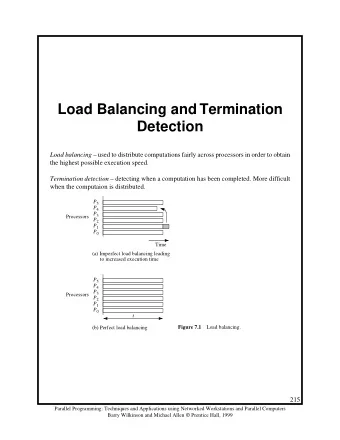
Load Balancing

Load Balancing

Load balancing: distributing data and/or computations across multiple processes to maximize efficiency for a parallel program.

◮ Static load-balancing: the algorithm decides a priori how to

divide the workload.

◮ Dynamic load-balancing: the algorithm collects statistics while

it runs and uses that information to rebalance the workload across the processes as it runs.

Static Load Balancing

◮ Round-robin: Hand the tasks in round robin fashion. ◮ Randomized: Divide the tasks in a randomized manner to help

load balance.

◮ Recursive bisection: Recursively divide a problem into

sub-problems of equal computational effort.

◮ Heuristic techniques: For example, a genetic algorithm to

determine a good static load balanced workload.

Dynamic Load Balancing

Manages a queue of tasks, known as the workpool.

◮ Usually more effective than static load balancing. ◮ Overhead of collecting statistics while the program runs. ◮ More complex to implement.

Dynamic Load Balancing

Manages a queue of tasks, known as the workpool.

◮ Usually more effective than static load balancing. ◮ Overhead of collecting statistics while the program runs. ◮ More complex to implement.

Two styles of dynamic load balancing:

◮ Centralized Workpool: The workpool is kept at a coordinator

process, which hands out tasks and collects newly generated tasks from worker processes.

◮ Distributed Workpool: The workpool is distributed across the

worker processes. Tasks are exchanged between arbitrary

• processes. Requires a more complex termination detection

technique to know when the program has finished.

Centralized Workpool

worker processes Task 2 1

. . .

task queue

Request task new tasks/ Return results/

Coordinator P Centralized Work Pool

p−1 p−2

◮ The workpool holds a collection of tasks to be performed. Processes

are supplied with tasks when they finish previously assigned task and request for another task. This leads to load balancing. Processes can generate new tasks to be added to the workpool as well.

Centralized Workpool

worker processes Task 2 1

. . .

task queue

Request task new tasks/ Return results/

Coordinator P Centralized Work Pool

p−1 p−2

◮ The workpool holds a collection of tasks to be performed. Processes

are supplied with tasks when they finish previously assigned task and request for another task. This leads to load balancing. Processes can generate new tasks to be added to the workpool as well.

◮ Termination: The workpool program is terminated when

◮ the task queue is empty, and ◮ each worker process has made a request for another task without any

new tasks being generated.

Distributed Workpool

Distributed task queue Requests/Tasks

◮ The task of queues is distributed across the processes. ◮ Any process can request any other process for a task or send it a task. ◮ Suitable when the memory required to store the tasks is larger than

can fit on one system.

Distributed Workpool

How does the work load get balanced?

◮ Receiver initiated: A process that is idle or has light load asks

another process for a task. Works better for a system with high load.

◮ Sender initiated: A process that has a heavy load send task(s) to

another process. Works better for a system with a light load. How do we determine which process to contact?

◮ Round robin. ◮ Random polling. ◮ Structured: The processes can be arranged in a logical ring or a tree.

Distributed Workpool Termination

Two conditions must be true to be able to terminated a distributed workpool correctly:

◮ local termination conditions exist on each process, and ◮ no messages are in transit.

This is tricky....here are two ways to deal with it:

Distributed Workpool Termination

Two conditions must be true to be able to terminated a distributed workpool correctly:

◮ local termination conditions exist on each process, and ◮ no messages are in transit.

This is tricky....here are two ways to deal with it:

◮ Tree-based termination algorithm. A tree order is imposed on the

processes based on who sends a message for the first time to a

• process. At termination the tree is traversed bottom-up to the root.

◮ Dual-pass token ring algorithm. A separate phase that passes a token

to determine if the distributed algorithm has finished. The algorithm specifically detects if any messages were in transit.

Dual-pass Token Ring Termination

Pj Pi Pn−1 Task Pi turns white token black P white token white token

◮ Process 0 becomes white when terminated and passes a “white”

token to process 1.

◮ Processes pass on the token after meeting local termination

• conditions. However, if a process send a message to a process earlier

than itself in the ring, it colors itself black. A black process colors a token “black” before passing it on. A white process passes the token without any change.

◮ If process 0 receives a “white” token, termination conditions have

been met. If it receives a “‘black” token, it starts a new ring with another “white token.”

Example: Shortest Paths

◮ Given a directed graph with n vertices and m weighted edges, find the

shortest paths from a source vertex to all other vertices.

◮ For two given vertices i and j, the weight of the edge between the

two is given by the weight function w(i, j). The distance is infinite if there is no edge between i and j.

Example: Shortest Paths

◮ Given a directed graph with n vertices and m weighted edges, find the

shortest paths from a source vertex to all other vertices.

◮ For two given vertices i and j, the weight of the edge between the

two is given by the weight function w(i, j). The distance is infinite if there is no edge between i and j.

◮ Graph can be represented in two different ways:

◮ Adjacency matrix: A two dimensional array w[0 . . . n − 1][0 . . . n − 1]

holds the weight of the edges.

◮ Adjacency lists: An array adj[0 . . . n − 1] of lists, with the ith list

represents the vertices adjacent to the ith vertex. The list stores the weights of the corresponding edges.

Example: Shortest Paths

◮ Given a directed graph with n vertices and m weighted edges, find the

shortest paths from a source vertex to all other vertices.

◮ For two given vertices i and j, the weight of the edge between the

two is given by the weight function w(i, j). The distance is infinite if there is no edge between i and j.

◮ Graph can be represented in two different ways:

◮ Adjacency matrix: A two dimensional array w[0 . . . n − 1][0 . . . n − 1]

holds the weight of the edges.

◮ Adjacency lists: An array adj[0 . . . n − 1] of lists, with the ith list

represents the vertices adjacent to the ith vertex. The list stores the weights of the corresponding edges.

◮ Sequential shortest paths algorithms

◮ Dijstkra’s shortest paths algorithm: Uses a priority queue to grow the

shortest paths tree one edge at a time: has limited opportunities for parallelism.

◮ Moore’s shortest path algorithm: Works by finding new shorter paths

all over the graph. Allows for more parallelism but can do extra work by exploring a given vertex multiple times.

Moore’s Algorithm

◮ A FIFO queue of vertices to explore is maintained. Initially it contains

just the source vertex.

Moore’s Algorithm

◮ A FIFO queue of vertices to explore is maintained. Initially it contains

just the source vertex.

◮ A distance array dist[0 . . . n − 1] represents the current shortest

distance to the respective vertex. Initially the distance to the source vertex is zero and all other distances are infinity.

Moore’s Algorithm

◮ A FIFO queue of vertices to explore is maintained. Initially it contains

just the source vertex.

◮ A distance array dist[0 . . . n − 1] represents the current shortest

distance to the respective vertex. Initially the distance to the source vertex is zero and all other distances are infinity.

◮ Remove the vertex i in the front of the queue and explore edges from

• it. Suppose vertex j is connected to vertex i. Then compare the

shortest distance from the source that is currently known to the distance going through vertex i. If the new distance is shorter, update the distance and add vertex j into the queue (if not in queue already).

j i d[j] d[i] w(i,j)

Moore’s Algorithm

◮ A FIFO queue of vertices to explore is maintained. Initially it contains

just the source vertex.

◮ A distance array dist[0 . . . n − 1] represents the current shortest

distance to the respective vertex. Initially the distance to the source vertex is zero and all other distances are infinity.

◮ Remove the vertex i in the front of the queue and explore edges from

• it. Suppose vertex j is connected to vertex i. Then compare the

shortest distance from the source that is currently known to the distance going through vertex i. If the new distance is shorter, update the distance and add vertex j into the queue (if not in queue already).

j i d[j] d[i] w(i,j)

◮ Repeat until the vertex queue is empty.

Shortest Paths using Centralized Workpool

◮ Task (for Shortest paths): One vertex to be explored. ◮ Coordinator process (process 0): Holds the workpool, which

consists of the queue of vertices to be explored. This queue shrinks and grows dynamically.

Centralized Workpool Pseudo-Code

centralized shortest paths(s, w, n, p, id) // id: current process id, total p processes, numbered 0, . . . , p − 1 // s - source vertex, w[0..n-1][0..n-1] - weight matrix, dist[0..n-1] shortest distance // Q - queue of vertices to explore, initially empty coordinator ← 0 bcast(w, &n, coordinator); // the coordinator part if (id = coordinator) numWorkers ← 0 enqueue(Q, s) do recv(Pany, &worker, ANY TAG, &tag) if (tag = NEW TASK TAG) recv(&j, &newdist, Pany, &worker, NEW TASK TAG) dist[j] ← min(dist[j], newdist[j]) enqueue(Q, j) else if tag = INIT TAG or tag = REQUEST TAG if (tag = REQUEST TAG) numWorkers ← numWorkers - 1 if (queueNotEmpty(Q)) v ← dequeue(Q) send(&v, Pworker, TASK TAG) send(dist, &n, Pworker, TASK TAG) numWorkers ← numWorkers + 1 while (numWorkers > 0) for i ← 1 to p-1 do send(&dummy, Pworker, TERMINATE TAG)

Centralized Workpool Pseudo-Code (contd.)

else //the worker part send(&id, Pcoordinator, INIT TAG) recv(&v, Pcoordinator, ANY TAG, &tag) while tag = TERMINATE TAG) recv(dist, &n, Pcoordinator, TASK TAG) for j ← 0 to n-1 do if w[v][j] = ∞ newdist j ← dist[v] + w[v][j] if newdist j < dist[j] dist[j] ← newdist j send(&id, Pcoordinator, NEW TASK TAG) send(&j, &newdist j, Pcoordinator, NEW TASK TAG) send(&id, Pcoordinator, REQUEST TAG) recv(&v, Pcoordinator, ANY TAG, &tag)

Improvements to the Centralized Workpool Solution

◮ Make the task contain multiple vertices to make the

granularity be more coarse.

◮ Instead of sending a new task every time a lower distance is

found, wait until all edges out of a vertex have been explored and then send results together in one message.

◮ Updating local copy of distance array would eliminate many

tasks from being created in the first place. This would give further improvement.

◮ Use a priority queue instead of a FIFO queue for workpool.

This should give some more improvement for large enough graphs.

Shortest Paths using Distributed Workpool

◮ Process i searches around vertex i and stores if vertex i is in

the queue or not.

◮ Process i keeps track of the ith entry of the distance array. ◮ Process i stores the adjacency matrix row or adjacency list for

vertex i. If a process receives a message containing a distance, it checks with its stored value and if it is smaller, it updates distances to its neighbors and send messages to the corresponding processes

Improvements to the Distributed Workpool Solution

◮ Make the task contain multiple vertices to make the

granularity be more coarse.

◮ Combine messages and only send known minimums by

keeping a local estimate of the distance array.

◮ Maintain the local copy of the distance array as a priority

queue. In actual practice, the distributed workpool solution (with the

• ptimizations) was able to scale much more than the centralized

solution.

Comparison of Various Implementations

$

Further Reading

◮ Pencil Beam Redefinition Algorithm: A dynamic load

balancing scheme that is adaptive in nature. The statistics are collected centrally but the data is rebalanced in a distributed manner! This is based on an actual medical application code.

◮ Parallel Toolkit Library: Masters project by Kirsten Allison.

This library gives a centralized and distributed workpool design pattern that any application programmer can use without having to implement the same complex patterns again and again. Notes on both are on the class website under lecture notes.