Load Balancing Load Balancing: Example Example Problem Consider 6 - PowerPoint PPT Presentation
Load Balancing Load Balancing: Example Example Problem Consider 6 jobs whose processing times is given as follows Input: m identical machines, n jobs with i th job having processing time t i Jobs 1 2 3 4 5 6 Goal: Schedule jobs to
Load Balancing Load Balancing: Example Example Problem Consider 6 jobs whose processing times is given as follows Input: m identical machines, n jobs with i th job having processing time t i Jobs 1 2 3 4 5 6 Goal: Schedule jobs to computers such that t i 2 3 4 6 2 2 ◮ Jobs run contiguously on a machine ◮ A machine processes only one job a time Consider the following schedule on 3 machines ◮ Makespan or maximum load on any machine is minimized 3 6 2 5 Definition 1 4 Let A ( i ) be the set of jobs assigned to machine i . The load on i is T i = � j ∈ A ( i ) t j . The loads are: T 1 = 8, T 2 = 5, and T 3 = 6. So makespan of The makespan of A is T = max i T i schedule is 8 Load Balancing is NP-Complete Greedy Algorithm 1. Consider the jobs in some fixed order 2. Assign job j to the machine with lowest load so far Example Decision version: given n , m and t 1 , t 2 , . . . , t n and a target T , is there a schedule with makespan at most T ? Jobs 1 2 3 4 5 6 2 3 4 6 2 2 t i Problem is NP-Complete: reduce from Subset Sum. 3 6 2 5 1 4
Putting it together Optimality for each machine i T i = 0 (* initially no load *) A ( i ) = ∅ (* initially no jobs *) Problem for each job j Is the greedy algorithm optimal? No! For example, on Let i be machine with smallest load A ( i ) = A ( i ) ∪ { j } (* schedule j on i *) T i = T i + t j (* compute new load *) Jobs 1 2 3 4 5 6 t i 2 3 4 6 2 2 Running Time the greedy algorithm gives schedule with makespan 8, but optimal is 7 ◮ First loop takes O ( m ) time In fact, the load balancing problem is NP -complete. ◮ Second loop has O ( n ) iterations ◮ Body of loop takes O (log m ) time using a priority heap ◮ Total time is O ( n log m + m ) Quality of Solution Bounding the Optimal Value Lemma T ∗ ≥ max j t j , where T ∗ is the optimal makespan Theorem (Graham 1966) Proof. The makespan of the schedule output by the greedy algorithm is at most 2 times the optimal make span. In other words, the greedy Some machine will run the job with maximum processing time algorithm is a 2-approximation. Lemma T ∗ ≥ 1 j t j , where T ∗ is the optimal makespan Challenge � m How do we compare the output of the greedy algorithm with the Proof. optimal? How do we get the value of the optimal solution? ◮ Total processing time is � j t j ◮ We will obtain bounds on the optimal value ◮ Some machine must do at least 1 m (or average) of the total work
Analysis of Greedy Algorithm Tightness of Analysis Proposition Theorem The analysis of the greedy algorithm is tight, i.e., there is an The greedy algorithm is a 2-approximation example on which the greedy schedule has twice the optimal Proof. makespan Let machine i have the maximum load T i , and let j be the last job Proof. scheduled on machine i Consider problem of m ( m − 1) jobs with processing time 1 and the ◮ At the time j was scheduled, machine i must have had the last job with processing time m . least load; load on i before assigning job j is T i − t j Greedy schedule: distribute first the m ( m − 1) jobs equally among ◮ Since i has the least load, we know T i − t j ≤ T k , for all k . the m machines, and then schedule the last job on machine 1, Thus, m ( T i − t j ) ≤ � k T k giving a makespan of ( m − 1) + m = 2 m − 1 ℓ t ℓ . So T i − t j ≤ 1 k T k = 1 ℓ t ℓ ≤ T ∗ ◮ But � k T k = � � � The optimal schedule: run last job on machine 1, and then m m ◮ Finally, T i = ( T i − t j ) + t j ≤ T ∗ + T ∗ = 2 T ∗ distribute remaining jobs equally among m − 1 machines, giving a makespan of m Improved Greedy Algorithm Technical Lemma Modified Greedy Lemma Sort the jobs in descending order of processing time, and process If there are more than m jobs then T ∗ ≥ 2 t m +1 jobs using greedy algorithm Proof. for each machine i Consider the first m + 1 jobs T i = 0 (* initially no load *) ◮ Two of them must be scheduled on same machine, by A ( i ) = ∅ (* initially no jobs *) pigeon-hole principle for each job j in descending order of processing time Let i be machine with smallest load ◮ Both jobs have processing time at least t m +1 , since we A ( i ) = A ( i ) ∪ { j } (* schedule j on i *) consider jobs according to processing time, and this proves the T i = T i + t j (* compute new load *) lemma
Analysis of Modified Greedy Tightness of Analysis Theorem The modified greedy algorithm is a 3 / 2 -approximation Proof. Theorem (Graham) Once again let i be the machine with highest load, and let j be the Modified greedy is a 4 / 3 -approximation last job scheduled The 4 / 3-analysis is tight. ◮ If machine i has only one job then schedule is optimal ◮ If i has at least 2 jobs, then it must be the case that j ≥ m + 1. This means t j ≤ t m +1 ≤ 1 2 T ∗ ◮ Thus, T i = ( T i − t j ) + t j ≤ T ∗ + 1 2 T ∗ (Weighted) Set Cover Problem Greedy Rule Input Given a set U of n elements, a collection S 1 , S 2 , . . . S m of subsets of U , with weights w i Goal Find a collection C of these sets S i whose union is ◮ Pick the next set in the cover to be the one that makes “most equal to U and such that � i ∈C w i is minimized. progress” towards the goal ◮ Covers many (uncovered) elements Example ◮ Has a small weight Let U = { 1 , 2 , 3 , 4 , 5 , 6 , 7 , 8 } , with ◮ If R is the set of elements that aren’t covered as yet, add set w i S i to the cover, if it minimizes the quantity | S i ∩ R | S 1 = { 1 } w 1 = 1 S 2 = { 2 } w 2 = 1 S 3 = { 3 , 4 } w 3 = 1 S 4 = { 5 , 6 , 7 , 8 } w 4 = 1 S 5 = { 1 , 3 , 5 , 7 } w 5 = 1 + ǫ S 6 = { 2 , 4 , 6 , 8 } w 6 = 1 + ǫ { S 5 , S 6 } is a set cover of weight 2 + 2 ǫ
Greedy Algorithm Example: Greedy Algorithm 1 + ǫ 1 + ǫ Initially R = U and C = ∅ 1 1 while R � = ∅ Example let S i be the set that minimizes w i / | S i ∩ R | C = C ∪ { i } Let U = { 1 , 2 , 3 , 4 , 5 , 6 , 7 , 8 } , with R = R \ S i 1 return C S 1 = { 1 } S 2 = { 2 } S 3 = { 3 , 4 } S 4 = { 5 , 6 , 7 , 8 } Running Time S 5 = { 1 , 3 , 5 , 7 } S 6 = { 2 , 4 , 6 , 8 } 1 ◮ Main loop iterates for O ( n ) time, where | U | = n w 1 = w 2 = w 3 = w 4 = 1 and w 5 = w 6 = 1 + ǫ ◮ Minimum S i can be found in O (log m ) time, using a priority Greedy Algorithm first picks S 4 , then S 3 , and heap, where there are m sets in set cover instance finally S 1 and S 2 ◮ Total time is O ( n log m ) Cost for covering an element Cost of element: Example Example Let U = { 1 , 2 , 3 , 4 , 5 , 6 , 7 , 8 } , with Definition ◮ Suppose the greedy algorithm selects sets S 1 , S 2 , . . . S k (in S 1 = { 1 } S 2 = { 2 } that order) to form the set cover. S 3 = { 3 , 4 } S 4 = { 5 , 6 , 7 , 8 } ◮ Consider an element s that is first covered when S i is picked S 5 = { 1 , 3 , 5 , 7 } S 6 = { 2 , 4 , 6 , 8 } ◮ Let R be the set of elements that are uncovered when S i is w 1 = w 2 = w 3 = w 4 = 1 and w 5 = w 6 = 1 + ǫ . The greedy picked algorithm picks S 4 , S 3 , S 2 , S 1 in that order. The costs of elements ◮ The cost of covering s is c s = w ( S i ) / | S i ∩ R | , where w ( S i ) is are given as follows weight of the set S i c 1 = 1 c 2 = 1 c 3 = 1 / 2 c 4 = 1 / 2 c 5 = 1 / 4 c 6 = 1 / 4 c 7 = 1 / 4 c 8 = 1 / 4
Costs of Covers and Elements Bounding costs of sets Lemma For every set S k , � s ∈ S k c s ≤ H ( | S k | ) · w k , where H ( n ) = � n 1 i = Θ( ln n ) Proposition i =1 If C is the set cover computed by the greedy algorithm then Proof. � i ∈C w i = � s ∈ U c s Let S k = { s 1 , . . . s d } , where s i is covered before s j if i ≤ j Proof left as exercise ◮ Consider the iteration when s j is covered; at this time Main Idea R ⊇ { s j , s j +1 , . . . s d } � s ∈ Sk c s Upper bound the ratio , i.e., to say “to cover a lot of cost, ◮ Average progress cost of S k is w k / | S k ∩ R | ≤ w k / ( d − j + 1) w k you need to use a lot of weight” ◮ Suppose s j gets covered because S i is selected by greedy w i w k w k algorithm. Then, c s j = | S i ∩ R | ≤ | S k ∩ R | ≤ d − j +1 s ∈ S k c s = � d j =1 c s j ≤ � d w i ◮ Hence, � d − j +1 = H ( d ) w k j =1 Analysis of the Greedy Algorithm Tightness of Analysis Theorem The greedy algorithm for set cover is a H ( d ∗ ) -approximation, where d ∗ = max i | S i | Analysis Tight? Does the Greedy Algorithm give better approximation guarantees? Proof. No! Let C ∗ be the optimal set cover, and C the set cover computed by Consider a generalization of the set cover example. Each column greedy algorithm has 2 k − 1 elements, and there are two sets consisting of a column 1 ◮ By previous lemma we know w i ≥ � s ∈ S i c s i and so we each with weight 1 + ǫ . Additionally there are log n sets of H ( d ∗ ) have w ∗ = � 1 i ∈C ∗ w i ≥ � � s ∈ S i c s i increasing size of weight 1. The greedy algorithm will pick these i ∈C ∗ H ( d ∗ ) ◮ Further, � log n sets given weight log n , while the best cover has weight 2 + 2 ǫ � s ∈ S i c s ≥ � s ∈ U c s i ∈C ∗ ◮ Thus, w ∗ = � 1 i ∈C ∗ w i ≥ � � s ∈ S i c s i ≥ i ∈C ∗ H ( d ∗ ) 1 1 � s ∈ U c s = � i ∈C w i H ( d ∗ ) H ( d ∗ )
Best Algorithm for Set Cover Theorem If P � = NP then no polynomial time algorithm can achieve a better than H ( n ) approximation. Proof beyond the scope of this course.
Recommend
More recommend
Explore More Topics
Stay informed with curated content and fresh updates.


