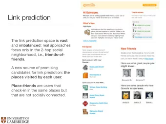
Link Prediction 1 Motivation Recommending new friends in - PowerPoint PPT Presentation

SimRank … … IJCAI Q : What is most related Philip S. Yu KDD conference to ICDM? Ning Zhong ICDM R. Ramakrishnan SDM M. Jordan AAAI … NIPS … Author Conference 31

SimRank PKDD SDM PAKDD 0.008 0.007 0.009 KDD 0.005 ICML 0.011 ICDM 0.005 0.004 CIKM ICDE 0.005 0.004 0.004 ECML SIGMOD DMKD 32

Methods for Link Prediction: based on paths 1. Shortest paths 2. Katz 3. Hitting and commute time 4. Rooted page rank 5. SimRank 33

Methods for Link Prediction: other Low rank approximations M adjacency matrix , represent M with a lower rank matrix M k Apply SVD (singular value decomposition) The rank-k matrix that best approximates M 34

Singular Value Decomposition  σ  v    1 1      σ v          2 T 2 A  U Σ V  u u u  1 2 r            [ n × r ] [ r × r ] [ r × n ] σ v     r r • r : rank of matrix A • σ 1 ≥ σ 2 ≥ … ≥σ r : singular values (square roots of eig-vals AA T , A T A)    u , u , , u • : left singular vectors (eig-vectors of AA T )  1 2 r    v , v , , v •  : right singular vectors (eig-vectors of A T A) 1 2 r       • T T T A  σ u v  σ u v   σ u v  1 1 1 2 2 2 r r r

Methods for Link Prediction: other Unseen Bigrams Unseen bigrams: pairs of word that co-occur in a test corpus, but not in the corresponding training corpus Not just score(x, y) but score(z, y) for nodes z that are similar to ( δ ) the δ nodes most related to x x --- S x 36

Methods for Link Prediction : High-level approaches Clustering  Compute score(x, y) for al edges in E old  Delete the (1-p) fraction of the edges whose score is the lowest, for some parameter p  Recompute score(x, y) for all pairs in the subgraph 37

How to Evaluate the Prediction (outline) Each link predictor p outputs a ranked list L p of pairs in V × V − E old : predicted new collaborations in decreasing order of confidence In this paper, focus on Core, thus E ∗ new = E new ∩ (Core × Core) = |E ∗ new | Evaluation method: Size of the intersection of  the first n edge predictions from L p that are in Core × Core, and  the set E ∗ new  How many of the (relevant) top-n predictions are correct (precision?) 38

Evaluation: baseline Baseline: random predictor Randomly select pairs of authors who did not collaborate in the training interval Probability that a random prediction is correct: In the datasets, from 0.15% (cond-mat) to 0.48% (astro-ph) 39

Evaluation: Factor improvement over random 40

Evaluation: Factor improvement over random 41

Evaluation: Average relevance performance (random)  average ratio over the five datasets of the given predictor's performance versus a baseline predictor's performance.  the error bars indicate the minimum and maximum of this ratio over the five datasets.  the parameters for the starred predictors are: (1) for weighted Katz, β = 0.005; (2) for Katz clustering, β 1 = 0.001; ρ = 0.15; β 2 = 0.1; (3) for low-rank inner product, rank = 256; (4) for rooted Pagerank, α = 0.15; (5) for unseen bigrams, unweighted, common neighbors with δ = 8; and (6) for SimRank, C ( γ) = 0.8. 42

Evaluation: Average relevance performance (distance) 43

Evaluation: Average relevance performance (neighbors) 44

Evaluation: prediction overlap  How much similar are the predictions made by the different methods? Why? correct 45

Evaluation: datasets  How much does the performance of the different methods depends on the dataset?  (rank) On 4 of the 5 datasets best at an intermediate rank On qr-qc, best at rank 1, does it have a “simpler” structure”?  On hep-ph, preferential attachment the best  Why is astro-ph “difficult”? The culture of physicists and physics collaboration 46

Evaluation: small world The shortest path even in unrelated disciplines is often very short Basic classifier on graph distances does not work 47

Evaluation: restricting to distance three Many pairs of authors separated by a graph distance of 2 will not collaborate and Many pairs who collaborate are at distance greater than 2 Disregard all distance 2 pairs (do not just “close” triangles) 48

Evaluation: the breadth of data Three additional datasets 1. Proceedings of STOC and FOCS 2. Papers for Citeseer 3. All five of the arXiv sections Common neighbors vs Random  Suggests that is easier to predict links within communities 49

Extensions  Improve performance. Even the best (Katz clustering on gr-qc) correct on only about 16% of its prediction  Improve efficiency on very large networks (approximation of distances)  Treat more recent collaborations as more important  Additional information (paper titles, author institutions, etc) To some extent latently present in the graph 50

Outline  Estimating a score for each edge (seminal work of Liben- Nowell&Kleinberg  Neighbors measures, Distance measures, Other methods  Evaluation  Classification approach  Twitter 51

Using Supervised Learning Given a collection of records ( training set ) Each record contains a set of attributes (features) + the class attribute . Find a model for the class attribute as a function of the values of other attributes. Goal: previously unseen records should be assigned a class as accurately as possible. A test set is used to determine the accuracy of the model. Usually, the given data set is divided into training and test sets, with training set used to build the model and test set used to validate it. 52

Illustrating the Classification Task Learning Tid Attrib1 Attrib2 Attrib3 Class 1 Yes Large 125K No algorithm 2 No Medium 100K No No 3 No Small 70K 4 Yes Medium 120K No Induction 5 No Large 95K Yes 6 No Medium 60K No Learn 7 Yes Large 220K No Model Yes 8 No Small 85K 9 No Medium 75K No 10 No Small 90K Yes Model 10 Training Set Apply Model Tid Attrib1 Attrib2 Attrib3 Class 11 No Small 55K ? 12 Yes Medium 80K ? Deduction ? 13 Yes Large 110K 14 No Small 95K ? 15 No Large 67K ? 10 Test Set 53

Classification Techniques • Decision Tree based Methods • Rule-based Methods • Memory based reasoning • Neural Networks • Naïve Bayes and Bayesian Belief Networks • Support Vector Machines • Logistic Regression 54

Example of a Decision Tree Splitting Attributes Tid Refund Marital Taxable Cheat Status Income 1 Yes Single 125K No Refund 2 No Married 100K No Yes No 3 No Single 70K No 4 Yes Married 120K No NO MarSt Yes 5 No Divorced 95K Married Single, Divorced 6 No Married 60K No TaxInc NO 7 Yes Divorced 220K No < 80K > 80K 8 No Single 85K Yes 9 No Married 75K No NO YES 10 No Single 90K Yes 10 Model: Decision Tree Training Data 55

Classification for Link Prediction Class? Features (predictors)? PropFlow: random walks, stops at l or when cycle 56

Using Supervised Learning: why?  Even training on a single feature may outperform ranking (restriction to n-neighborhoods)  Dependencies between features 57

How to split the graph to get train data  tx length of computing features – ty length of determining the class attribute  Large tx => better quality of features as the network reaches saturation  Increasing ty increases positives 58

Imbalance  Sparse networks: |E| = k |V| for constant k << |V| The class imbalance ratio for link prediction in a sparse network is Ω (|V|/1) when at most |V| nodes are added Missing links is |V| 2 Positives V Treat each neighborhood as a separate problem 59

Metrics for Performance Evaluation Confusion Matrix: PREDICTED CLASS Class=Yes Class=No Class=Yes TP FN ACTUAL Class=No FP TN CLASS  TP TN  Accuracy    TP TN FP FN 60

ROC Curve TPR (sensitivity)=TP/(TP+FN) (percentage of positive classified as positive) FPR = FP/(TN+FP) (percentage of negative classified as positive) • (0,0): declare everything to be negative class • (1,1): declare everything to be positive class • (0,1): ideal Diagonal line: Random guessing Below diagonal line : prediction is opposite of the true class AUC: area under the ROC 61

Results Ensemble of classifiers: Random Forest Random forest: Ensemble classifier that constructs a multitude of decision trees at training time and output the class that is the mode (most frequent) of the classes (classification) or mean prediction (regression) of the individual trees. 62

Results 63

Outline  Estimating a score for each edge (seminal work of Liben- Nowell&Kleinberg  Neighbors measures, distance measures, other methods  Evaluation  Classification approach  Brief background on classification  Issues  The who to follow service at Twitter  Some practical considerations  Overall architecture of a real social network  SALSA (yet another link analysis algorithm  Some evaluation issues 64

Introduction Wtf (“Who to Follow"): the Twitter user recommendation service  Twitter: 200 million users, 400 million tweets every day (as of early 2013) http://www.internetlivestats.com/twitter-statistics/  Twitter needs to help existing and new users to discover connections to sustain and grow  Also used for search relevance, discovery, promoted products, etc. 65

Introduction Difference between:  Interested in  Similar to Is it a “social” network as Facebook? 66

The Twitter graph  Node: user (directed) edge: follows  Statistics (August 2012)  over 20 billion edges (only active users)  power law distributions of in-degrees and out-degrees.  over 1000 with more than 1 million followers,  25 users with more than 10 million followers. http://blog.ouseful.info/2011/07/07/visualising-twitter-friend-connections-using-gephi-an-example-using- wireduk-friends-network/ 67

The Twitter graph: storage  Stored in a graph database called FlockDB which uses MySQL as the underlying storage engine  Sharding and replication by a framework called Gizzard  Both custom solutions developed internally but open sourced  FlockDB holds the “ground truth" for the state of the graph  Optimized for low-latency, high-throughput reads and writes, and efficient intersection of adjacency lists (needed to deliver @- replies, or messages targeted to a specific user received mutual followers of the sender and recipient )  hundreds of thousands of reads per second and tens of thousands of writes per second . 68

The Twitter graph: analysis • Instead of simple get/put queries, many graph algorithms involve large sequential scans over many vertices followed by self-joins (for example, to materialize egocentric follower neighborhoods) • not time sensitive unlike graph manipulations tied directly to user actions (adding a follower) which have tight latency bounds. OLAP (online analytical processing) vs. OLTP (online transaction processing) analytical workloads that depend on sequential scans vs. short, primarily seek-based workloads that provide an interactive service 69

The Twitter graph: analysis • Instead of simple get/put queries, many graph algorithms involve large sequential scans over many vertices followed by self-joins (for example, to materialize egocentric follower neighborhoods) • not time sensitive unlike graph manipulations tied directly to user actions (adding a follower) which have tight latency bounds. OLAP (online analytical processing) vs. OLTP (online transaction processing) analytical workloads that depend on sequential scans vs. short, primarily seek-based workloads that provide a user-facing service 70

History of WTF 3 engineers, project started in spring 2010, product delivered in summer 2010 Basic assumption: the whole graph fits into memory of a single server 71

Design Decisions: To Hadoop or not? Case study: MapReduce implementation of PageRank • Each iteration a MapReduce job • Serialize the graph as adjacency lists for each vertex , along with the current PageRank value. • Mappers process all vertices in parallel: for each vertex on the adjacency list, the mapper emits an intermediate key-value pair: (destination vertex, partial PageRank) • Gather all key-value pairs with the same destination vertex, and each Reducer sums up the partial PageRank contributions • Convergence requires dozens of iterations. A control program sets up the MapReduce job, waits for it to complete, and checks for convergence by reading in the updated PageRank vector and comparing it with the previous. • This basic structure can be applied to a large class of “message -passing" graph (e.g., breadth-first search) 72

Design Decisions: To Hadoop or not? Shortcomings of MapReduce implementation of PageRank  MapReduce jobs have relatively high startup costs (in Hadoop, on a large, busy cluster, can be tens of seconds) , this places a lower bound on iteration time.  Scale-free graphs , whose edge distributions follow power laws, create stragglers in the reduce phase. (e.g., the reducer assigned to google.com) Combiners and other local aggregation techniques help  Must shuffle the graph structure (i.e., adjacency lists) from the mappers to the reducers at each iteration. Since in most cases the graph structure is static, wasted effort (sorting, network traffic, etc.).  The PageRank vector is serialized to HDFS , along with the graph structure, at each iteration. Excellent fault tolerance, but at the cost of performance. 73

Design Decisions: To Hadoop or not? Besides Hadoop: Improvements: HaLoop Twister, and PrIter Alternatives:  Google's Pregel implements the Bulk Synchronous Parallel model : computations at graph vertices that dispatch “messages " to other vertices. Processing proceeds in supersteps with synchronization barriers between each.  GraphLab and its distributed variant: computations either through an update function which defines local computations (on a single vertex) or through a sync mechanism which defines global aggregation in the context of different consistency models. 74

Design Decisions: To Hadoop or not? Decided to build their own system Hadoop reconsidered:  new architecture completely on Hadoop  in Pig a high-level dataflow language for large, semi-structured datasets compiled into physical plans executed on Hadoop  Pig Latin primitives for projection, selection, group, join, etc. Why not some other graph processing system? For compatibility, e.g., to use existing analytics hooks for job scheduling, dependency management, etc. 75

Overall Architecture 76

Overall Architecture: Flow 1. Daily snapshots of the Twitter graph imported from FlockDB into the Hadoop data warehouse 2. The entire graph loaded into memory onto the Cassovary servers, each holds a complete copy of the graph in memory. 3. Constantly generate recommendations for users consuming from a distributed queue containing all Twitter users sorted by a “last refresh" timestamp (~500 ms per thread to generate ~100 recommendations for a user) 4. Output from the Cassovary servers inserted into a sharded MySQL database, called, WTF DB. 5. Once recommendations have been computed for a user, the user is enqueued again with an updated timestamp. Active users who consume (or are estimated to soon exhaust) all their recommendations are requeued with much higher priority; typically, these users receive new suggestions within an hour. 77

Overall Architecture: Flow Graph loaded once a day, what about new users? Link prediction for new users  Challenging due to sparsity: their egocentric networks small and not well connected to the rest of the graph (cold start problem)  Important for social media services: user retention strongly affected by ability to find a community with which to engage.  Any system intervention is only effective within a relatively short time window. (if users are unable to find value in a service, they are unlikely to return) 1. new users are given high priority in the Cassovary queue, 2. a completely independent set of algorithms for real-time recommendations, specifically targeting new users. 78

Algorithms  Asymmetric nature of the follow relationship (other social networks e.g., Facebook or LinkedIn require the consent of both participating members)  Directed edge case is similar to the user-item recommendations problem where the “item” is also a user. 79

Algorithms: SALSA SALSA (Stochastic Approach for Link-Structure Analysis) a variation of HITS As in HITS hubs authorities HITS  Good hubs point to good authorities  Good authorities are pointed by good hubs hub weight = sum of the authority weights of the authorities pointed to by the hub   h a i j  j : i j authority weight = sum of the hub weights that   point to this authority. a h authorities hubs i j  j : j i 80

Algorithms: SALSA Random walks to rank hubs and authorities  Two different random walks (Markov chains): a chain of hubs and a chain of authorities  Each walk traverses nodes only in one side by traversing two links in each step h->a-h, a->h->a Transition matrices of each Markov chain: H and A W: the adjacency of the directed graph W r : divide each entry by the sum of its row W c : divide each entry by the sum of its column T H = W r W c T W r A = W c authorities hubs Proportional to the degree 81

Algorithms: Circle of trust Circle of trust: the result of an egocentric random walk (similar to personalized (rooted) PageRank)  Computed in an online fashion (from scratch each time) given a set of parameters (# of random walk steps, reset probability, pruning settings to discard low probability vertices, parameters to control sampling of outgoing edges at vertices with large out-degrees, etc.)  Used in a variety of Twitter products, e.g., in search and discovery, content from users in one's circle of trust upweighted 82

Algorithms: SALSA Hubs: 500 top-ranked nodes from the user's circle of trust Authorities: users that the hubs follow Hub vertices: user similarity (based on homophily, also useful) Authority vertices : “interested in" user recommendations. 83

Algorithms: SALSA How it works SALSA mimics the recursive nature of the problem:  A user u is likely to follow those who are followed by users that are similar to u.  A user is similar to u if the user follow the same (or similar) users. I. SALSA provides similar users to u on the LHS and similar followings of those on the RHS. II. The random walk ensures equitable distribution of scores in both directions III. Similar users are selected from the circle of trust of the user through personalized PageRank. 84

Evaluation  Offline experiments on retrospective data  Online A/B testing on live traffic Various parameters may interfere:  How the results are rendered (e.g., explanations)  Platform (mobile, etc.)  New vs old users 85

Evaluation: metrics Follow-through rate (FTR) (precision)  Does not capture recall  Does not capture lifecycle effects (newer users more receptive, etc. )  Does not measure the quality of the recommendations: all follow edges are not equal Engagement per impression (EPI): After a recommendation is accepted, the amount of engagement by the user on that recommendation in a specified time interval called the observation interval. 86

Extensions  Add metadata to vertices (e.g., user profile information) and edges (e.g., edge weights, timestamp, etc.)  Consider interaction graphs (e.g., graphs defined in terms of retweets, favorites, replies, etc.) 87

Extensions Two phase algorithm  Candidate generation : produce a list of promising recommendations for each user, using any algorithm  Rescoring : apply a machine-learned model to the candidates, binary classification problem (logistic regression) First phase: recall + diversity Second phase: precision + maintain diversity 88

References D. Liben-Nowell, and J. Kleinberg, The link-prediction problem for social networks. Journal of the American Society for Information Science and Technology, 58(7) 1019 – 1031 (2007) R. Lichtenwalter, J. T. Lussier, N. V. Chawla: New perspectives and methods in link prediction . KDD 2010: 243-252 G. Jeh, J. Widom: SimRank: a measure of structural-context similarity . KDD 2002: 538-543 P-N Tan, . Steinbach, V. Kumar. Introduction to Data Mining (Chapter 4) P. Gupta, A. Goel, J. Lin, A. Sharma, D. Wang, R.Zadeh. WTF: The Who to Follow Service at Twitter, WWW 2013 R. Lempel, S. Moran: SALSA: the stochastic approach for link-structure analysis . ACM Trans. Inf. Syst. 19(2): 131-160 (2001) 89

Extra slides 90

Design Decisions: How much memory? in-memory processing on a single server Why? 1. The alternative (a partitioned, distributed graph processing engine) significantly more complex and difficult to build, 2. It was feasible (72GB -> 144GB, 5 bytes per edge (no metadata); 24-36 months lead time) • In memory – not uncommon (google indexes + Facebook, Twitter many cache servers • A single machine • Graph distribution still hard (hash partitioning, minimize the number of edges that cross-partition (two stage, over partition #clusters>>#servers, still skew problems), use replication to provide n-hop guarantee (all n- neighbors in a singe site) • Avoids extra protocols (e.g., replication for fault-tolerance) 91

Overall Architecture: Cassovary In memory graph processing engine, written in Scala  Once loaded into memory, graph is immutable  Fault tolerance provided by replication, i.e., running many instances of Cassovary, each holding a complete copy of the graph in memory.  Access to the graph via vertex-based queries such as retrieving the set of outgoing edges for a vertex and sampling a random outgoing edge.  Multi-threaded: each query is handled by a separate thread.  Graph stored as optimized adjacency lists: the adjacency lists of all vertices in large shared arrays plus indexes (start, length) into these shared arrays  No compression  Random walks implemented using the Monte-Carlo method,  the walk is carried out from a vertex by repeatedly choosing a random outgoing edge and updating a visit counter.  Slower than a standard matrix-based implementation, but low runtime memory overhead 92

Algorithms: SALSA  Reduces the problem of HITS with tightly knit communities (TKC effect)  Better for single-topic communities  More efficient implementation 93

HITS and the TKC effect • The HITS algorithm favors the most dense community of hubs and authorities – Tightly Knit Community (TKC) effect

HITS and the TKC effect • The HITS algorithm favors the most dense community of hubs and authorities – Tightly Knit Community (TKC) effect 1 1 1 1 1 1

HITS and the TKC effect • The HITS algorithm favors the most dense community of hubs and authorities – Tightly Knit Community (TKC) effect 3 3 3 3 3

HITS and the TKC effect • The HITS algorithm favors the most dense community of hubs and authorities – Tightly Knit Community (TKC) effect 3 2 3 2 3 2 3 ∙2 3∙2 3∙2

HITS and the TKC effect • The HITS algorithm favors the most dense community of hubs and authorities – Tightly Knit Community (TKC) effect 3 3 3 3 3 3 3 2 ∙ 2 3 2 ∙ 2

HITS and the TKC effect • The HITS algorithm favors the most dense community of hubs and authorities – Tightly Knit Community (TKC) effect 3 4 3 4 3 4 3 2 ∙ 2 2 3 2 ∙ 2 2 3 2 ∙ 2 2

HITS and the TKC effect • The HITS algorithm favors the most dense community of hubs and authorities – Tightly Knit Community (TKC) effect 3 2n 3 2n after n iterations weight of node p is 3 2n proportional to the number of (BF) n paths that leave 3 n ∙ 2 n node p 3 n ∙ 2 n 3 n ∙ 2 n