Link prediction via matrix factorization Charles Elkan University - PowerPoint PPT Presentation

Link prediction via matrix factorization Charles Elkan University of California, San Diego September 6, 2011 1 / 26

Outline Introduction: Three related prediction tasks 1 Link prediction in networks 2 Discussion 3 2 / 26

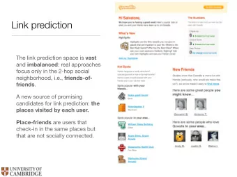
Link prediction Given current friendship edges, predict future edges. Application: Facebook. Popular method: Scores computed from graph topology, e.g. betweenness. 3 / 26

Collaborative filtering Given ratings of movies by users, predict other ratings. Application: Netflix. Popular method: Matrix factorization. 4 / 26

Item response theory Given answers by students to exam questions, predict performance on other questions. Applications: Adaptive testing, diagnosis of skills. Popular method: Latent trait (i.e. hidden feature) models. 5 / 26

Dyadic prediction in general Given labels for some pairs of items (some dyads), predict labels for other pairs. What if we have side-information, e.g. mobility data for people in a social network? 6 / 26

Matrix factorization Associate latent feature values with each user and movie. Each rating is the dot-product of corresponding latent vectors. Learn the most predictive vector for each user and movie. 7 / 26

Side-information solves the cold-start problem Standard : All users and movies have training data. Cold-start users : No ratings for 50 random users. Double cold-start : No ratings for 50 random users and their movies. 1.2000 1.0000 0.9608 0.8039 0.8000 0.7451 Test set MAE 0.7162 0.7063 0.7118 0.6000 Baseline LFL 0.4000 0.2000 0.0000 Standard Cold-start users Cold-start users + movies Setting 8 / 26

Outline Introduction: Three related prediction tasks 1 Link prediction in networks 2 Discussion 3 9 / 26

Link prediction Link prediction : Given a partially observed graph, predict whether or not edges exist for the unknown-status dyads. ? ? ? ? Classic methods are unsupervised (non-learning) scores, e.g. betweenness, common neighbors, Katz, Adamic-Adar. 10 / 26

The bigger picture Solve a predictive problem. ◮ Contrast: Non-predictive task, e.g. community detection. Maximize objective defined by an application, e.g. AUC. ◮ Contrast: Algorithm but no goal function, e.g. betweenness. Learn from all available data. ◮ Contrast: Use only graph structure, e.g. commute time. Allow hubs, overlapping groups, etc. ◮ Contrast: Clusters, modularity. Make training time linear in number of edges. ◮ Contrast: MCMC, betweenness, SVD. Compare accuracy to best current results. ◮ Contrast: Compare only to classic methods. 11 / 26

Combined latent/explicit feature approach Each node’s identity influences its linking behavior. The identity of a node determines its latent features. Nodes also can have side-information predictive of linking. ◮ For author-author linking, side-information can be words in authors’ papers. Edges may also possess side-information. ◮ For country-country conflict, side-information is geographic distance, trade volume, etc. 12 / 26

Latent feature model LFL model for binary link prediction has parameters ◮ latent vectors α i ∈ R k for each node i ◮ scaling factors Λ ∈ R k × k ◮ weights W ∈ R d × d for node features ◮ weights v ∈ R d ′ for edge features. Node i has features x i , dyad ij has features z ij . Predicted label is ˆ G ij = σ ( α T i Λ α j + x T i Wx j + v T z ij ) 1 for sigmoid function σ ( x ) = 1+exp( − x ) . 13 / 26

Latent feature training True label is G ij , predicted label is ˆ G ij . Minimize regularized training loss: ℓ ( G ij , ˆ � min G ij ) + Ω( α, Λ , W, v ) α, Λ ,W,v ( i,j ) ∈O Sum is only over known edges and known non-edges. Stochastic gradient descent (SGD) converges quickly. 14 / 26

Challenge: Class imbalance Vast majority of node-pairs do not link with each other. Area under ROC curve (AUC) is standard performance measure. For a random pair of positive and negative examples, AUC is the probability that the positive one has higher score. ◮ Not influenced by relative size of positive and negative classes. Models trained to maximize accuracy are suboptimal. ◮ Sampling is popular, but loses information. ◮ Weighting is merely heuristic. 15 / 26

Optimizing AUC Empirical AUC counts concordant pairs � AUC ∝ 1 [ f p − f q > 0] p ∈ + ,q ∈− Train LFL model to maximize approximation to AUC: � ℓ ( ˆ G ij − ˆ min G ik , 1) + Ω( α, Λ , W, v ) α, Λ ,W,v ( i,j,k ) ∈D where D = { ( i, j, k ) : G ij = 1 , G ik = 0 } . With stochastic gradient descent, a fraction of one epoch is enough for convergence. 16 / 26

Experimental comparison Compare ◮ latent features versus unsupervised scores ◮ latent features versus explicit features. Datasets from applications of link prediction: ◮ Computational biology : Protein-protein interaction network, metabolic interaction network ◮ Citation networks : NIPS authors, condensed matter physicists ◮ Social phenomena : Military conflicts between countries, U.S. electric power grid, multiclass relationships. 17 / 26

Multiclass link prediction Alyawarra dataset has kinship relations for 104 people { brother, sister, father, . . . } . LFL outperforms Bayesian models, even infinite ones. 18 / 26

Binary link prediction datasets nodes |O + | |O − | + ve: − ve ratio mean degree Prot-Prot 2617 23710 6,824,979 1 : 300 9.1 Metabolic 668 5564 440,660 1 : 80 8.3 NIPS 2865 9466 8,198,759 1 : 866 3.3 Condmat 14230 2392 429,232 1 : 179 0.17 Conflict 130 320 16580 1 : 52 2.5 PowerGrid 4941 13188 24,400,293 1 : 2000 2.7 Protein-protein interaction data from Noble. Per protein: 76 features. Metabolic interactions of S. cerevisiae from the KEGG/PATHWAY database. Per protein: 157 phylogenetic features, 145 gene expression features, 23 location features. NIPS. Per author: 100 LSI features from vocabulary of 14,035 words. Condensed-matter physicists [Newman]. Use node-pairs 2 hops away in first five years. Military disputes [MID 3.0]. Per country: population, GDP, polity. Per dyad: 6 features, e.g. geographic distance. US electric power grid network [Watts and Strogatz]. 19 / 26

Latent features versus unsupervised scores Latent features are more predictive of linking behavior. 20 / 26

Learning curves Unsupervised scores need many edges to be known. Latent features are predictive with fewer known edges. For the military conflicts dataset: 21 / 26

Latent features combined with side-information Difficult to infer latent structure more predictive than side-information. But combining the two is beneficial: 22 / 26

Related paper in Session 19, Thursday am Kernels for Link Prediction with Latent Feature Models , Nguyen and Mamitsuka, ECML 2011. Fruit fly protein-protein interaction network, 2007 data. Connected component with minimum degree 8: 701 nodes (713). 100 latent features, tenfold CV: AUC 0.756 + / − 0.012. Better than IBP (0.725), comparable to kernel method. 23 / 26

Outline Introduction: Three related prediction tasks 1 Link prediction in networks 2 Discussion 3 24 / 26

If time allowed Scaling up to Facebook-size datasets: better AUC than supervised random walks. Predicting labels for nodes, e.g. who will play Farmville (within network/collective/semi-supervised classification). 25 / 26

Conclusions Many prediction tasks involve pairs of entities: collaborative filtering, friend suggestion, and more. Learning latent features always gives better accuracy than any non-learning method. The most accurate predictions combine latent features with explicit features of nodes and of dyads. You don’t need EM, variational Bayes, MCMC, infinite number of parameters, etc. 26 / 26

References I 27 / 26