Linear Regression Implementation from Scratch Linear Regression - PowerPoint PPT Presentation

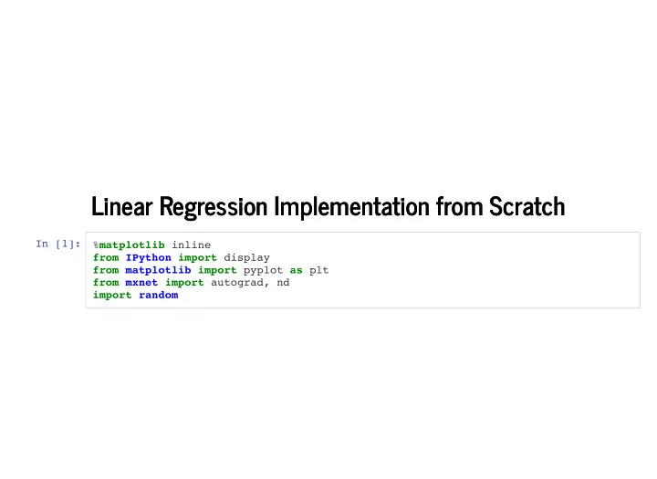
Linear Regression Implementation from Scratch Linear Regression Implementation from Scratch In [1]: % matplotlib inline from IPython import display from matplotlib import pyplot as plt from mxnet import autograd, nd import random

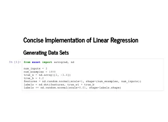
Generating Data Sets Generating Data Sets Randomly generate X ∈ ℝ 1000×2 Use ground truth: weight and bias w = [2, − 3.4] ⊤ b = 4.2 Generate label by with noise obeying a normal distribution with y = Xw + b + ϵ ϵ a mean of 0 and a standard deviation of 0.01. In [2]: num_inputs = 2 num_examples = 1000 true_w = nd.array([2, -3.4]) true_b = 4.2 features = nd.random.normal(scale=1, shape=(num_examples, num_inputs)) labels = nd.dot(features, true_w) + true_b labels += nd.random.normal(scale=0.01, shape=labels.shape)

Visualize the Second Feature and Label Visualize the Second Feature and Label In [3]: display.set_matplotlib_formats('svg') plt.figure(figsize=(6, 3)) plt.scatter(features[:, 1].asnumpy(), labels.asnumpy(), 1);

Reading Data Reading Data Iterate over the data set and return batch_size (batch size) random examples every time.

In [4]: def data_iter(batch_size, features, labels): num_examples = len(features) indices = list(range(num_examples)) # The examples are read at random, in no particular order random.shuffle(indices) for i in range(0, num_examples, batch_size): j = nd.array(indices[i: min(i + batch_size, num_examples)]) yield features.take(j), labels.take(j) # The “take” function will then return the corresponding element based # on the indices

Print a Small Data Batch Print a Small Data Batch In [5]: batch_size = 10 for X, y in data_iter(batch_size, features, labels): print(X, y) break [[ 1.7782049 0.17127965] [-0.2433725 -0.5560082 ] [-0.99795526 0.17728646] [-0.41475967 -1.2982413 ] [-2.1107438 -1.5111811 ] [-1.8830644 -0.4991788 ] [ 0.11150214 -0.22487849] [ 0.9314184 -0.7470997 ] [-0.3884701 -2.0006752 ] [-1.0986379 1.691893 ]] <NDArray 10x2 @cpu(0)> [ 7.1776037 5.609725 1.5751892 7.7738857 5.1178493 2.1461306 5.191642 8.586297 10.234753 -3.7403975] <NDArray 10 @cpu(0)>

Initialize Model Parameters Initialize Model Parameters Weights are initialized to normal random numbers using a mean of 0 and a standard deviation of 0.01, with the bias set to zero. b In [6]: w = nd.random.normal(scale=0.01, shape=(num_inputs, 1)) b = nd.zeros(shape=(1,))

Attach Gradients to Parameters Attach Gradients to Parameters In [7]: w.attach_grad() b.attach_grad()

De�ne the Linear Model De�ne the Linear Model In [8]: def linreg(X, w, b): return nd.dot(X, w) + b

De�ne the Loss Function De�ne the Loss Function In [9]: def squared_loss(y_hat, y): return (y_hat - y.reshape(y_hat.shape)) ** 2 / 2

De�ne the Optimization Algorithm De�ne the Optimization Algorithm In [10]: def sgd(params, lr, batch_size): for param in params: param[:] = param - lr * param.grad / batch_size

Training Training

In [11]: lr = 0.1 # Learning rate num_epochs = 3 # Number of iterations net = linreg # Our fancy linear model loss = squared_loss # 0.5 (y-y')^2 w = nd.random.normal(scale=0.01, shape=(num_inputs, 1)) b = nd.zeros(shape=(1,)) w.attach_grad() b.attach_grad() for epoch in range(num_epochs): for X, y in data_iter(batch_size, features, labels): with autograd.record(): l = loss(net(X, w, b), y) # Minibatch loss in X and y l.backward() # Compute gradient on l with respect to [w,b] sgd([w, b], lr, batch_size) # Update parameters using their gradient train_l = loss(net(features, w, b), labels) print('epoch %d , loss %f ' % (epoch + 1, train_l.mean().asnumpy())) epoch 1, loss 0.000049 epoch 2, loss 0.000050 epoch 3, loss 0.000049

Evaluate the Trained Model Evaluate the Trained Model In [12]: print('Error in estimating w', true_w - w.reshape(true_w.shape)) print('Error in estimating b', true_b - b) print(w) print(b) Error in estimating w [-0.00051641 0.00074124] <NDArray 2 @cpu(0)> Error in estimating b [-0.00073719] <NDArray 1 @cpu(0)> [[ 2.0005164] [-3.4007413]] <NDArray 2x1 @cpu(0)> [4.200737] <NDArray 1 @cpu(0)>