Linear mixed models fitted with lmer() in R : p values based on a - PowerPoint PPT Presentation

Contents Outline The Kenward–Roger improvement of the F –statistic Parametric bootstrap (PB) Final comparison Final rem Linear mixed models fitted with lmer() in R : p –values based on a Kenward-Roger modification of the F-statistic or on parametric bootstrap methods. Ulrich Halekoh and Søren Højsgaard Department of Molecular Biology and Genetics Aarhus University, Denmark 10. august 2011 1 / 24

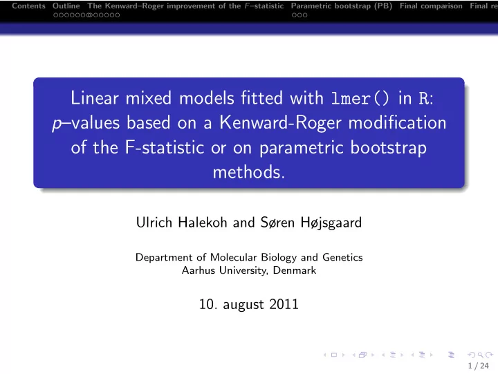
Contents Outline The Kenward–Roger improvement of the F –statistic Parametric bootstrap (PB) Final comparison Final rem 1 Outline Motivation: Sugar beets - A split–plot experiment Motivation: A random regression problem Our goal 2 The Kenward–Roger improvement of the F –statistic An“F” –statistic 3 Parametric bootstrap (PB) Finding a Bartlett correction using PB Small simulation study: A random regression problem 4 Final comparison 5 Final remarks 2 / 24

Contents Outline The Kenward–Roger improvement of the F –statistic Parametric bootstrap (PB) Final comparison Final rem Motivation: Sugar beets - A split–plot experiment Dependence of yield [kg] and sugar percentage of sugar beets on harvest time and sowing time is investigated. Five sowing times and two harvesting times were used. The experiment was laid out in three blocks. Experimental plan for sugar beets experiment Sowing times: 1: 4/4, 2: 12/4, 3: 21/4, 4: 29/4, 5: 18/5 Harvest times: 1: 2/10, 2: 21/10 Plot allocation: | Block 1 | Block 2 | Block 3 | +-----------|-----------|-----------+ Plot | 1 1 1 1 1 | 2 2 2 2 2 | 1 1 1 1 1 | Harvest time 1-15 | 3 4 5 2 1 | 3 2 4 5 1 | 5 2 3 4 1 | Sowing time |-----------|-----------|-----------| Plot | 2 2 2 2 2 | 1 1 1 1 1 | 2 2 2 2 2 | Harvest time 16-30 | 2 1 5 4 3 | 4 1 3 2 5 | 1 4 3 2 5 | Sowing time +-----------|-----------|-----------+ 3 / 24

Contents Outline The Kenward–Roger improvement of the F –statistic Parametric bootstrap (PB) Final comparison Final rem Motivation: Sugar beets - A split–plot experiment Let h denote harvest time ( h = 1 , 2), b denote block ( b = 1 , 2 , 3) and s denote sowing time ( s = 1 , . . . , 5). Let H = 2, B = 3 and S = 5. For simplicity we assume that there is no interaction between sowing and harvesting times. A typical model for such an experiment would be: y hbs = µ + α h + β b + γ s + U hb + ǫ hbs , (1) where U hb ∼ N (0 , ω 2 ) and ǫ hbs ∼ N (0 , σ 2 ). Notice that U hb describes the random variation between whole–plots (within blocks). 4 / 24

Contents Outline The Kenward–Roger improvement of the F –statistic Parametric bootstrap (PB) Final comparison Final rem Motivation: Sugar beets - A split–plot experiment As the design is balanced we may make F–tests for each of the effects as: R-code > beets$bh <- with(beets, interaction(block, harvest)) > summary(aov(sugpct~block+sow+harvest+Error(bh), beets)) Error: bh Df Sum Sq Mean Sq F value Pr(>F) block 2 0.0327 0.0163 2.58 0.28 harvest 1 0.0963 0.0963 15.21 0.06 Residuals 2 0.0127 0.0063 Error: Within Df Sum Sq Mean Sq F value Pr(>F) sow 4 1.01 0.2525 101 5.7e-13 Residuals 20 0.05 0.0025 Notice: the F–statistics are F 1 , 2 for harvest time and F 4 , 20 for sowing time. 5 / 24

Contents Outline The Kenward–Roger improvement of the F –statistic Parametric bootstrap (PB) Final comparison Final rem Motivation: Sugar beets - A split–plot experiment Using lmer() from lme4 we can fit the models and test for no effect of sowing and harvest time as follows: R-code > beetLarge<-lmer(sugpct~block+sow+harvest+(1|block:harvest), + data=beets, REML=FALSE) > beet_no.harv <- update(beetLarge, .~.-harvest) > beet_no.sow <- update(beetLarge, .~.-sow) > as.data.frame(anova(beetLarge, beet_no.sow)) Df AIC BIC logLik Chisq Chi Df Pr(>Chisq) beet_no.sow 6 -2.795 5.612 7.398 NA NA NA beetLarge 10 -79.997 -65.985 49.999 85.2 4 1.374e-17 > as.data.frame(anova(beetLarge, beet_no.harv)) Df AIC BIC logLik Chisq Chi Df Pr(>Chisq) beet_no.harv 9 -69.08 -56.47 43.54 NA NA NA beetLarge 10 -80.00 -65.99 50.00 12.91 1 0.0003262 The LRT based p –values are anti–conservative: the effect of harvest appears stronger than it is. 6 / 24

Contents Outline The Kenward–Roger improvement of the F –statistic Parametric bootstrap (PB) Final comparison Final rem Motivation: A random regression problem Random coefficient model The change with age of the distance between two cranial fissures was observed for 16 boys and 11 girls from age 8 until age 14. 8 9 10 11 12 13 14 Male Female 30 distance 25 20 8 9 10 11 12 13 14 age 7 / 24

Contents Outline The Kenward–Roger improvement of the F –statistic Parametric bootstrap (PB) Final comparison Final rem Motivation: A random regression problem Random coefficient model Plot suggests: dist [ i ] = α sex [ i ] + β sex [ i ] age [ i ] + A Subj [ i ] + B Subj [ i ] age [ i ] + e [ i ] with ( A , B ) ∼ N (0 , S ). ML-test of β boy = β girl : R-code > ort1ML<- lmer(distance ~ age + Sex + age:Sex + (1 + age | Subject), + REML = FALSE, data=Orthodont) > ort2ML<- update(ort1ML, .~.-age:Sex) > as.data.frame(anova(ort1ML, ort2ML)) Df AIC BIC logLik Chisq Chi Df Pr(>Chisq) ort2ML 7 446.8 465.6 -216.4 NA NA NA ort1ML 8 443.8 465.3 -213.9 5.029 1 0.02492 8 / 24

Contents Outline The Kenward–Roger improvement of the F –statistic Parametric bootstrap (PB) Final comparison Final rem Our goal Our goal... Our goal is to improve on the tests provided by lmer() . There are two issues here: The choice of test statistic and The reference distribution in which the test statistic is evaluated. 9 / 24

Contents Outline The Kenward–Roger improvement of the F –statistic Parametric bootstrap (PB) Final comparison Final rem Setting the scene For multivariate normal data Y n × 1 ∼ N ( X n × p β p × 1 , Σ ) we consider the test of the hypothesis L l × p β = β 0 where L is a regular matrix of estimable functions of β . The linear hypothesis can be tested via the Wald-type statistic F = 1 l ( ˆ σ ) L ) − 1 L ( ˆ β − β 0 ) ⊤ L ⊤ ( L ⊤ Φ ( ˆ β − β 0 ) (2) Φ = ( X ⊤ Σ X ) − 1 : the asymptotic covariance matrix of the REML estimate ˆ β , σ : vector of REML estimates of the elements of Σ ˆ 10 / 24

Contents Outline The Kenward–Roger improvement of the F –statistic Parametric bootstrap (PB) Final comparison Final rem An “F” –statistic Kenward and Roger’s modification Kenward and Roger (1997) modify the test statistic Φ is replaced by an improved small sample approximation Φ A Furthermore the statistic is scaled by a factor λ denominator degrees of freedom m are determined such that the approximate expectation and variance are those of a F l , m distribution. 11 / 24

Contents Outline The Kenward–Roger improvement of the F –statistic Parametric bootstrap (PB) Final comparison Final rem An “F” –statistic Restriction on covariance If Σ is linear combination of known matrices G i � Σ = σ i G i (3) i then Φ A ( ˆ σ ) is dependent only on the first partial deriviatives of Σ − 1 : ∂ Σ − 1 = − Σ − 1 ∂ Σ ∂σ i Σ − 1 . ∂σ i Notice: Variance component and random coefficient models satisfy this restriction. Φ A ( ˆ σ ) depends also on Var ( ˆ σ ). Kenward and Roger propose to estimate Var ( ˆ σ ) via the inverse expected information matrix. 12 / 24

Contents Outline The Kenward–Roger improvement of the F –statistic Parametric bootstrap (PB) Final comparison Final rem An “F” –statistic R package lme4 The R package lme4 (Bates, D., Maechler, M, Bolker, B., 2011) provides efficient estimation of linear mixed models. The package provides all necessary matrices and estimates to implement the Kenward-Roger approach. 13 / 24

Contents Outline The Kenward–Roger improvement of the F –statistic Parametric bootstrap (PB) Final comparison Final rem An “F” –statistic Properties of the Kenward–Roger adjustment The modification of the F-statistic by Kenward and Roger yields the exact F-statistic in case of Hotelling multivariate T–test and for ANOVA-models which allow exact F–statistics. Simulation studies (e.g. Spilke, J. et al.(2003)) indicate that the Kenward-Roger approach perform mostly better than alternatives (like Satterthwaite or containment method) for blocked experiments even with missing data. 14 / 24

Contents Outline The Kenward–Roger improvement of the F –statistic Parametric bootstrap (PB) Final comparison Final rem An “F” –statistic Kenward–Roger: split-plot (sugar-beets) The Kenward–Roger approach yields the same results as the anova-test: R-code > beetLarge <- update(beetLarge, REML=TRUE) > beet_no.harv <- update(beet_no.harv, REML=TRUE) Test for harvest effect: R-code > KRmodcomp(beetLarge,beet_no.harv)$stats[c( ' df2 ' , ' Fstat ' , ' pval ' )] df2 Fstat pval 2.00038 15.20898 0.05988 15 / 24

Contents Outline The Kenward–Roger improvement of the F –statistic Parametric bootstrap (PB) Final comparison Final rem An “F” –statistic Kenward–Roger: random regression (cranial change) For the data on change in cranial distances the Kenward and Roger modified F-test yields R-code > ort1<- update(ort1ML, .~., REML = TRUE) > ort2<- update(ort2ML, .~., REML = TRUE) > KRmodcomp(ort1,ort2)$stats[c( ' df2 ' , ' pval ' )] df2 pval 24.99863 0.03262 The p-value form the ML-test was 0.0249. 16 / 24