Lecure 3: Models and measurements for thermal syste ms Types of - PowerPoint PPT Presentation

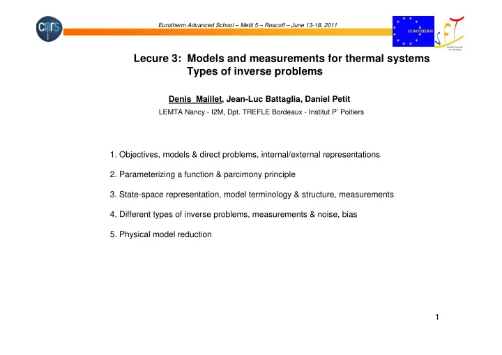
Eurotherm Advanced School – Metti 5 – Roscoff – June 13-18, 2011 Lecure 3: Models and measurements for thermal syste ms Types of inverse problems Denis Maillet , Jean-Luc Battaglia, Daniel Petit LEMTA Nancy - I2M, Dpt. TREFLE Bordeaux - Institut P’ Poitiers 1. Objectives, models & direct problems, internal/external representations 2. Parameterizing a function & parcimony principle 3. State-space representation, model terminology & structure, measurements 4. Different types of inverse problems, measurements & noise, bias 5. Physical model reduction 1

Eurotherm Advanced School – Metti 5 – Roscoff – June 13-18, 2011 1. Objectives of a mode l � (in heat transfer) First objective: Simulation of physical reality = Direct Problem u ( t ) : heat source/flux, variable external temperature : measured temperature at given time t and given location y : modelled temperature at given time t and given location y mo 2

Example: model of a semi infinite medium (1 input - 1 output) − k Perfect temperature sensor: y = y exact = y ( t ) T ( x , t ) Output equation: mo s = + y ( t ) y ( t ) y ( t ) Solution of direct problem: mo mo relax mo forced ∞ ( ) ( ) ∫ ∫ t = + − τ τ τ y ( t ) G x , x , t T ( x ) d x Z t u ( ) d External representation: mo s 0 0 0 convolution product Green’s function = / ρ c a k  ( ) 2 ( ) 2  1     − + ( ) 1 x x x x ( ) = exp − 2 / 4 ( ) Z t x a t exp s exp s =   −  +  −   G x , x, t s     s b π t 4 4 2 π a t a t a t c   = ρ b k       3

Perfect temperature sensor: y = y * zero initial Thermal impedance: temperature field 1 ( ) ( ) exp 2 / 4 = − Z t x a t s π b t ( ) 1 ( ) exp = Z p - x p / a s b p β ) x s p = Laplace parameter (s -1 ) ∞ ( ) ( ) ( ) ( ) ( ) ( ) ∫ with exp d = = − y p Z p u p f p f t pt t forced mo 0   a   Parameter list β = ( a , b , x s ) = β b Parameter « vector »      x  s ( ) 1 2 / 2 2 2 ⇒ β β β β = + + a b x b in J m -2 K -1 s -1/2 - x s in m a in W m -2 - s M of the white box type (internal representation) : internal parameters of physical nature 4

Semi-infinite medium model: general case { } = β x , u ( . ) , T 0 . ( ) List of data of Direct Problem:   a structural input initial   parameter (stimulus) state = β b vector     functions  x  s 5

2. Problem of function parameterizing & Parcimony principle ∞ ∑ { } = u ( t ) u f ( t ) � with f f j j 1 2 = j 1 function basis of infinite number of functions: [ 0 t sup ] → R on [ 0 t sup ] [ ] T f ( ) ( ) ( ) [ ] f = T u = u T � ⇒ = t f t f t � u u u ( t ) ( t ) 1 2 1 2 column vectors with an infinite number of components ∞ = ∑ ⇒ = u ( t ) u f ( t ) u u ( t ), f ( t ) j j j j = j 1 projection of u ( t ) onto f j ( t )   u truncation 1   = ∑ n u ≠   u ⇒ = u ( t ) u f ( t ) u ( t ) 2 u ( t ) replaced by in practice: param j j   � = j 1    u  n Good approximation: The model-builder has to choose 2 things: high n ⇒ large number of parameters 1) functions f j 2) their number n 6

Parameterization: 2 possible choices of local function basis n ∑ = u ( t ) u f ( t ) param j j = j 1 door functions hat functions 0 if t : local discretized value → interpolated u param ( t ) u u : averaged value over an interval j j • interesting for : • interesting for : β β ( T ) (P) u ( T ) T (P) u ( t ) 0 non uniform linear excitation initial 7 non linear temperature dependent heterogeneous temperature excitation thermophysical properties material

Parameterization (continued) Remarks non-local bases available: eigenfunctions f j of the heat equation • (method of separation of variables) = u param t ( ) Fourier series, for example t ∫ orthogonal bases (with a unit function norm N j ) interesting: sup = δ • f ( t ) f ( t ) d t N j k j j k t inf • non constant time step possible Extended parameter vector x • gathering the Direct Problem data:  β    { } x u = → = β x , u ( . ) , T 0 (P)   T     0 parameterized list functions 8

Parcimony principle: limitation of the number of parameters (or of degrees of freedom) to be sought inverter : beginner experienced constraint objectives: = parameters greediness: ideal realistic too many parameters sought parameterization parameterization / quality of measurements or available a priori information 9

3. State-space representation, model terminology & structure, measurements ( ) ∂ T k grad + = ρ + div T q c Boundary, interface and initial conditions ∂ vol t W/m 3 distributed parameter system = State of the system = continuous temperature field: T (P , t ) T ( t ) P [ ] T = � ( t ) T ( t ) T ( t ) T ( t ) Discretized state becoming = vector : 1 2 N in a N dimension space (number of nodes) T d lumped parameter system: E T U T T = = = ( t , , ) with ( t t 0 ) 0 d t [ ] U = Linear heat source (excitation): q vol (P, t ) T � ( t ) u ( t ), u ( t ) u p t ( ) 1 2 p excitated nodes [ ] U = T q vol ( T ( P, t )) � ( t ) u ( T ( t )), u ( T ( t )) u ( T p t ( )) Non-linear heat source: 1 2 p excitated nodes 10

State-space representation (continued) Case of a linear heat source with temperature independent thermophysical properties and coefficients E T U A T B U A B = + ( t , , ) with and : constant matrices (selection of observed nodes) 11

Output equation: detailed ( )  T t  1   ( ) T t   2   ( ) T t 3 q = 5 observed temperatures ( )  y t  0 0 0 0 1 0 0 0 0     � 1 mo ( ) T t       4 ( ) 0 0 0 0 0 0 0 0 0 y t (output) �   2   mo   ( ) T t 5   ( )   ( ) = y t = 0 0 0 0 0 0 0 0 0   y t � 3 mo mo      �  ( ) y t 0 0 0 0 0 0 0 0 0   �     4 mo N = 20 nodes ( ) T t     17   ( ) y t 0 0 0 0 0 1 0 0 0 �     5 mo  ( )  T t 18   ( ) T t   19   ( ) T t   20 12

T d A T B U = + Linear state equation : d t Explicit solution for temperature field: t ∫ T exp A T exp A B U = − + − τ τ τ ( t ) ( ( t t ) ) ( ( t ) ) ( ) d 0 0 t 0 and for model output: t ∫ y C exp A T C exp A B U = − + − τ τ τ ( t ) ( ( t t ) ) ( ( t ) ) ( ) d mo 0 0 t 0 Relaxation of initial state forced (convolution) response Remarks: - advection case possible (dispersion in porous medium, one-temperature model): ( ) ∂ T div λ grad − ρ grad + = ρ + Boundary, interface and initial conditions T c v . T q c vol f ∂ t - coupled modes transfer : radiation in semitransparent absorbing medium (Heat equation + radiative transfer equation) ⇒ composite state X : T   ( t ) Discretized temperature field: position X = ( t )   I  ( t )  Discretized intensity field: wavelength, direction, position 13

T T A B U y C A B U = − − ⇒ = − − d - steady state case (linear) : 1 1 A T B U = + = 0 mo d t Model terminology and structure Before parameterization After parameterization x = η = η y mo ( t , ) y mo ( t , x ) • single output: extended parameter scalar list scalar vector y = y x mo = η η ( t , x ) ( t , ) • multiple output: mo column extended parameter list column vector vector vector   β   { } = x u = , ( ) , 0 ( P ) . • data β x u T     T   0 η ( t , . ) or η η ( t , . ) : scalar or vector function η η = structure of the model x or x : corresponding data (list/vector) 14

Structure of a parameterized model in heat transfer Direct Problem Data dimensions of system parametrized shape thermophysical properties contact resistances heat transfer coefficients emissivities   β struct … = β   β   Model output pos location of detectors 15

Comparison between measurements and state model 16

Direct and inverse problems data y known x ? MODEL Direct problem : mo part of x ? known y Inverse problem : MODEL Objective of inverse problem: finding a part x r of x , using additional information (output y or something else)   β struct   β   x = pos Extended parameter vector:  U  ( t )   T   0 x   x sought ( r esearched) parameters = r   x   c omplementary part: known c 17