Lecture 9: Neural Networks (Part 1) Feb 25th, 2020 Lecturer: Steven - PDF document
CSCI 5525 Machine Learning Fall 2019 Lecture 9: Neural Networks (Part 1) Feb 25th, 2020 Lecturer: Steven Wu Scribe: Steven Wu We have just learned about kernel functions that allow us to implicitly lift the raw feature vector x to expanded
CSCI 5525 Machine Learning Fall 2019 Lecture 9: Neural Networks (Part 1) Feb 25th, 2020 Lecturer: Steven Wu Scribe: Steven Wu We have just learned about kernel functions that allow us to implicitly lift the raw feature vector x to expanded feature φ ( x ) that may lie in R ∞ . The kernel trick allows us to make linear predictions φ ( x ) ⊺ w without explicitly writing down the weight vector w . Note that the mapping φ is fixed after we choose the hyperparameters. Now we will talk about neural networks that were originally invented by Frank Rosenblatt. When neural network was first invented, it was called multi-layer perceptron . Similar to kernel, the approach of neural networks also makes prediction of the form φ ( x ) ⊺ w , but it explicitly learns the feature expansion mapping φ ( x ) . So how do we make an expressive feature mapping φ ? One natural idea is to take composition of linear functions. Warmup: composition of linear functions. • First linear transformation: x → W 1 x + b 1 • Second linear transformation: x → W 2 ( W 1 x + b 1 ) + b 2 • . . . . . . • L -th linear transformation: x → W L ( . . . ( W 1 x + b 1 ) . . . ) + b L Question: do we gain anything? Well, not quite. Observe that W L ( . . . ( W 1 x + b 1 ) . . . ) + b L = Wx + b, where W = W L . . . W 1 and b = b L + W L b L − 1 + . . . + W L . . . W 2 b 1 . 1 Non-linear activation To go beyond linear function, we will need to introduce “non-linearity” between the linear func- tions. Recall that in the lecture of logistic regression, we introduce a probability model 1 Pr [ Y = 1 | X = x ] = 1 + exp( − w ⊺ x ) ≡ σ ( w ⊺ x ) 1
where σ is the logistic or sigmoid function. See Figure 2. Now consider a vector-valued version that applies the logisitc function coordinate wise: f i ( z ) = σ ( W i z + b i ) . This gives the most basic neural network. x → ( f L ◦ · · · ◦ f 1 )( x ) , f i ( z ) = σ ( W i z + b i ) . where Here we call the { W i } L i =1 the weights , and { b i } L i =1 the biases . More generally, given a collection of activation (or nonlinearities, transfer, link ) functions { σ i } L i =1 , weights, and biases, we can write down a basic form of a neural network: F ( x, θ ) = σ L ( W L ( . . . W 2 σ 1 ( W 1 x + b 1 ) + b 2 . . . ) + b L ) where θ denotes the set of parameters W 1 , . . . , W L , b 1 , . . . , b L . DAG view. We can view a neural network as a directed acyclic graph (DAG). The input layer basically have each node corresponding to a single x i . See the illustration in Figure 1. In some applications, each x i might be vector-valued. For example, if x i corresponds to a pixel, it should contain 3 values. In this case, each W ij will also be a vector. Any layer that is not the input layer or the output layer is called a hidden layer . n O p o Wztb 4 8 23 2 EX EI hkxtbi.us oCZz Zz WzViVEfCZD be Figure 1: Graphical view of neural network. 1.1 Choices of activation functions. • Indicator or threshold: z → 1 [ z ≥ 0] • Sigmoid or logistic (Figure 2): 1 z → 1 + exp( − z ) 2
Figure 2: Logistic/sigmoid and hyperbolic functions Figure 3: ReLU and Leaky ReLU functions • Hyperbolic tangent: z → tanh( z ) • Rectificed linear unit (ReLU) (Figure 3): z → max { 0 , z } Variants include Leaky ReLU and ELU. These are the most popular choices now since the AlexNet paper [1], which kicked off the Deep Learning revolution. • Identity: z → z . This is often used in the last layer when we evaluate the loss. 2 Expressiveness It turns out this one hidden layer can already enable tremendously more representation power than a simple linear function. In fact, you can use such networks to approximate any “reasonable” functions according to the universal approximation theorem below. Theorem 2.1 (Universal approximation theorem) . Let f : R d → R be any continuous function. For any approximation error ǫ > 0 , there exists a set of parameters θ = ( W 1 , b 1 , W 2 , b 2 ) such that for any x ∈ [0 , 1] d | f ( x ) − ( W 2 σ ( W 1 x + b 1 ) + b 2 ) | ≤ ǫ where σ is a nonconstant, bounded, and continuous function (e.g. ReLU and logistic). 3
In other words, a single hidden layer neural network can approximate any continuous function to any degree of precision. However, such a neural network can be very wide, and even though it exists, we may not easily find it. More recently, there has been analogous universal approximation theorem with deep neural network with bounded widths that are essentially the dimension of the data [2]. Y n i ar l I l l l l l l l K w y X C t b fi Figure 4: Universal approximation theorem in the special case where x, f ( x ) ∈ R . On the left: the neural network graph in this case. On the right: intuition about the theorem. The continuous function f (in black) can be approximated a piecewise linear functions such that each piece is given by a weighted ReLU function (with an additive bias term). 3 Learning pipeline. • Split the data into traning and validation datasets. • Hyperparameters: pick a class of functions for the networks (or architecture), the function F ( · , · ) . • ERM: on training data set { ( x i , y i ) } , we pick a loss function ℓ (e.g. cross entropy loss function, square loss) and perform empirical risk minimization : n 1 � arg min ℓ ( y i , F ( x i , θ )) n θ i =1 • Choose the architecture with the lowest validation error. References [1] A. Krizhevsky, I. Sutskever, and G. E. Hinton. Imagenet classification with deep convolutional neural networks. In F. Pereira, C. J. C. Burges, L. Bottou, and K. Q. Weinberger, editors, 4
Advances in Neural Information Processing Systems 25 , pages 1097–1105. Curran Associates, Inc., 2012. [2] Z. Lu, H. Pu, F. Wang, Z. Hu, and L. Wang. The expressive power of neural networks: A view from the width. In I. Guyon, U. V. Luxburg, S. Bengio, H. Wallach, R. Fergus, S. Vish- wanathan, and R. Garnett, editors, Advances in Neural Information Processing Systems 30 , pages 6231–6239. Curran Associates, Inc., 2017. 5
Recommend
More recommend
Explore More Topics
Stay informed with curated content and fresh updates.
