Lecture 9: Demand Uncertainty: Demand Uncertainty: Lecture 9: - PDF document

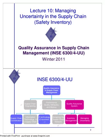
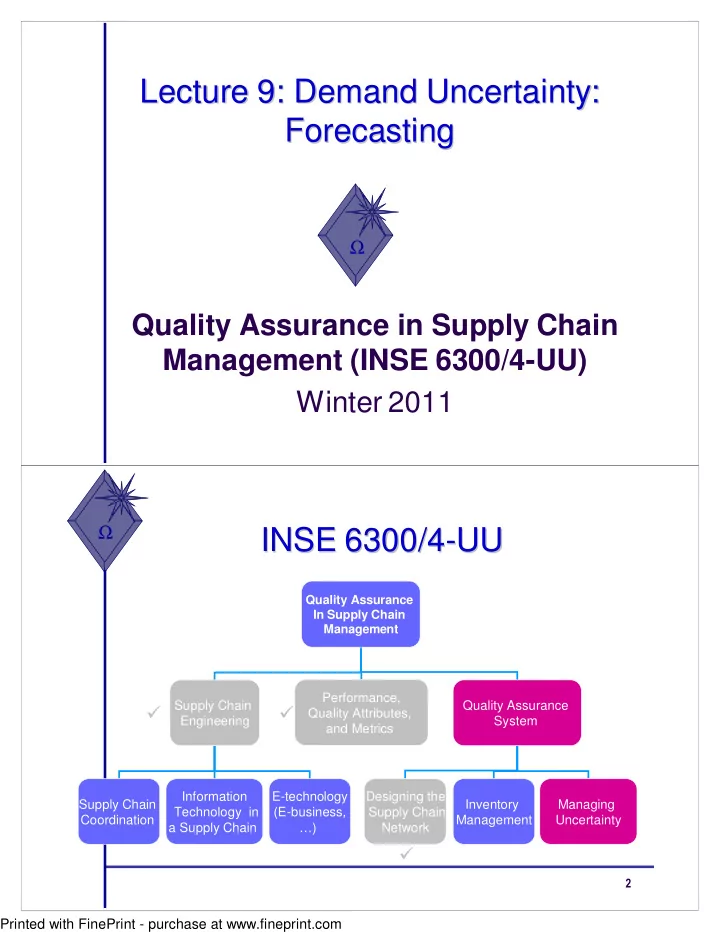
Lecture 9: Demand Uncertainty: Demand Uncertainty: Lecture 9: Forecasting Forecasting Ω Quality Assurance in Supply Chain Management (INSE 6300/4-UU) Winter 2011 Ω INSE 6300/4- -UU UU INSE 6300/4 Quality Assurance In Supply Chain Management Performance, Supply Chain Quality Assurance � � Quality Attributes, Engineering System and Metrics Information E-technology Designing the Supply Chain Inventory Managing Technology in (E-business, Supply Chain Coordination Management Uncertainty a Supply Chain …) Network � � Printed with FinePrint - purchase at www.fineprint.com

Ω Overview Overview � Forecasting: Role and Characteristics � Time Series Forecasting Methods � Measures of Forecast Error � Role of Forecasting Role of Forecasting Ω in a Supply Chain in a Supply Chain � The basis for all strategic and planning decisions in a supply chain � Used for both push and pull processes � Examples: � Production: scheduling, inventory, aggregate planning � Marketing: sales force allocation, promotions, new production introduction � Finance: plant/equipment investment, budgetary planning � Personnel: workforce planning, hiring, layoffs � All of these decisions are interrelated � Printed with FinePrint - purchase at www.fineprint.com

Ω Characteristics of Forecasts Characteristics of Forecasts � Forecasts are always wrong. Should include expected value and measure of error � Long-term forecasts are less accurate than short-term forecasts (forecast horizon is important) � Aggregate forecasts are more accurate than disaggregate forecasts � Ω Forecasting Methods Forecasting Methods � Qualitative: primarily subjective; rely on judgment and opinion � Time Series: use historical demand only � Static � Adaptive � Causal: use the relationship between demand and some other factor to develop forecast � Simulation � Imitate consumer choices that give rise to demand � Can combine time series and causal methods � Printed with FinePrint - purchase at www.fineprint.com

Basic Approach to Basic Approach to Ω Demand Forecasting Demand Forecasting � Understand the objectives of forecasting � Integrate demand planning and forecasting � Identify major factors that influence the demand forecast � Understand and identify customer segments � Determine the appropriate forecasting technique � Establish performance and error measures for the forecast � Components of an Components of an Observation Ω Observation Observed demand (O) = Systematic component (S) + Random component (R) Level (current deseasonalized demand) Trend (growth or decline in demand) Seasonality (predictable seasonal fluctuation) • Systematic component: Expected value of demand (Prediction) • Random component: The part of the forecast that deviates from the systematic component (Estimation) • Forecast error: difference between forecast and actual demand � Printed with FinePrint - purchase at www.fineprint.com

٠Overview Overview � � Forecasting: Role and Characteristics � Time Series Forecasting Methods � Measures of Forecast Error � Time Series Time Series ٠� A time series is a sequence of data points, measured typically at successive times, spaced at (often uniform) time intervals � Time series analysis comprises methods that attempt to understand such time series to understand the underlying theory of the data points � Where did they come from? what generated them?, � Time series method is used to make forecasts (predictions) �� Printed with FinePrint - purchase at www.fineprint.com

Time Series Time Series ٠� Time series prediction is the use of a model to predict future events based on known past events: � To predict future data points before they are measured � Two Main Goals: � (a) identifying the nature of the phenomenon represented by the sequence of observations, � (b) forecasting (predicting future values of the time series variable) � Both of these goals require that the pattern of observed time series data is identified and more or less formally described �� Time Series Time Series ٠� Once the pattern is established, we can interpret and integrate it with other data (i.e., use it in the theory of the investigated phenomenon, e.g., seasonal commodity prices) � Regardless of the depth of the understanding and the validity of the interpretation (theory) of the phenomenon, we can extrapolate the identified pattern to predict future events �� Printed with FinePrint - purchase at www.fineprint.com

٠Time Series Patterns Time Series Patterns �� Time Series Time Series ٠Forecasting Methods Forecasting Methods � Goal is to predict systematic component of demand � Multiplicative: (level)(trend)(seasonal factor) � Additive: level + trend + seasonal factor � Mixed: (level + trend)(seasonal factor) � Static methods � Adaptive forecasting �� Printed with FinePrint - purchase at www.fineprint.com

Ω Forecasting Methods Forecasting Methods � Static � Level, trend, and seasonality do not vary as new demand is observed � Estimation based on historical data � Using the same values for all future forecasts � Adaptive � Moving average � Simple exponential smoothing � Holt’s model ( with trend ) � Winter’s model ( with trend and seasonality ) �� Static Methods Static Methods Ω � Assume a mixed model: Systematic component = (level + trend)(seasonal factor) F t+l = [L + ( t + l )T] S t+l forecast in period t for demand in period t + l L = estimate of level during period 0 (the deseasonalized demand) T = estimate of trend (increase or decrease in demand) S t = estimate of seasonal factor for period t D t = actual demand in period t F t = forecast of demand in period t �� Printed with FinePrint - purchase at www.fineprint.com

٠Static Methods Static Methods � Three steps: � Estimating level and trend � Estimating seasonal factors � Estimating the forecast �� Time Series Forecasting Time Series Forecasting ٠Forecast demand for the Quarter Demand D t next four quarters. II, 1998 8000 III, 1998 13000 IV, 1998 23000 I, 1999 34000 II, 1999 10000 III, 1999 18000 IV, 1999 23000 I, 2000 38000 II, 2000 12000 III, 2000 13000 IV, 2000 32000 I, 2001 41000 �� Printed with FinePrint - purchase at www.fineprint.com

Time Series Forecasting Time Series Forecasting ٠50,000 40,000 30,000 20,000 10,000 0 97,2 97,3 97,4 98,1 98,2 98,3 98,4 99,1 99,2 99,3 99,4 00,1 �� Estimating Level and Trend Estimating Level and Trend ٠� Before estimating level and trend, demand data must be deseasonalized � Deseasonalized demand = demand that would have been observed in the absence of seasonal fluctuations (each season is given equal weight) � Periodicity ( p ) � The number of periods after which the seasonal cycle repeats itself � for demand at Tahoe Salt: p = 4 (average of demand of p consecutive periods) �� Printed with FinePrint - purchase at www.fineprint.com

Deseasonalizing Demand Deseasonalizing Demand Ω [D t-(p/2) + D t+(p/2) + Σ 2D i ] / 2p for p even (sum is from i = t+1-(p/2) to t-1+(p/2)) D t = Σ D i / p for p odd (sum is from i = t-[(p-1)/2] to t+[(p-1)/2]) The average of demand from period l+1 to l+p is the deseasonalized demand for l+(p+1)/2 �� Ω Deseasonalizing Demand Demand Deseasonalizing For the example, p = 4 is even For t = 3: D3 = {D1 + D5 + Sum(i=2 to 4) [2Di]}/8 = {8000+10000+[(2)(13000)+(2)(23000)+(2)(34000)]}/8 = 19750 D4 = {D2 + D6 + Sum(i=3 to 5) [2Di]}/8 = {13000+18000+[(2)(23000)+(2)(34000)+(2)(10000)]/8 = 20625 �� Printed with FinePrint - purchase at www.fineprint.com

٠Deseasonalizing Demand Demand Deseasonalizing �� Time Series of Demand Time Series of Demand ٠�� Printed with FinePrint - purchase at www.fineprint.com

٠Deseasonalizing Demand Demand Deseasonalizing Then include trend D t = L + t T where D t = deseasonalized demand in period t L = level (deseasonalized demand at period 0) T = trend (rate of growth of deseasonalized demand) Trend is determined by linear regression using deseasonalized demand as the dependent variable and period as the independent variable (can be done in Excel) (Tools-Data Analysis-Regression) �� ٠Linear Regression Linear Regression � linear regression is a regression method of modeling the conditional expected value of one variable y given the values of some other variable or variables x � Linear regression is called "linear" because the relation of the response to the explanatory variables is assumed to be a linear function of some parameters �� Printed with FinePrint - purchase at www.fineprint.com

٠Linear Regression Linear Regression Y = a + bX �� Deseasonalizing Demand Demand Deseasonalizing ٠In the example, � Input Y Range: C5:C12 � Input X Range: A5:A12 L = 18,439 and T = 524 �� Printed with FinePrint - purchase at www.fineprint.com