Adaptive Estimation of the Distribution Function and its Density in - PowerPoint PPT Presentation
Adaptive Estimation of the Distribution Function and its Density in Sup-Norm Loss Evarist Gin e and Richard Nickl Department of Mathematics University of Connecticut Let X 1 , ..., X n be i.i.d. with completely un- known law P on R .
Adaptive Estimation of the Distribution Function and its Density in Sup-Norm Loss Evarist Gin´ e and Richard Nickl Department of Mathematics University of Connecticut
→ Let X 1 , ..., X n be i.i.d. with completely un- known law P on R . → Define also P n = n − 1 � n i =1 δ X i , the mea- sure consisting of point masses at the obser- vations (’empirical measure’).
→ We want to find ’data-driven’ functions T ( y, X 1 , ..., X n ), y ∈ R , that optimally esti- mate � y (A) the distribution function F ( y ) = −∞ dP ( x ); (B) its density function f ( y ) = d dy F ( y ); in sup-norm loss on the real line.
Case (A) : A classical minimax result is √ nE sup lim inf inf sup | T n ( y ) − F ( y ) | ≥ c > 0 . n T n F y ∈ R → The natural candidate for T n is the sample � y cdf F n ( y ) = −∞ dP n ( t ), which is an efficient estimator of F in ℓ ∞ ( R ) . Case (B) : If f is contained in some H¨ older space C t ( R ) with norm � · � t , then one has t n (2 t +1) E � T n − f � ∞ ≥ c ( D ) > 0 � � lim n inf sup log n T n � f � t ≤ D
→ Clearly, the step function F n cannot be used to estimate the density f of F . → Can one outperform F n as an estimator for F in the sense that differentiable F can be estimated without knowing a priori that F is smooth? → Somewhat suprisingly maybe, the answer is yes .
Theorem 1 (Gin´ e, Nickl (2008, PTRF)) Let X 1 , ..., X n be i.i.d. on R with unknown law P . Then there exists a purely-data driven estimator ˆ F n ( s ) that satisfies √ n � � ˆ F n − F � ℓ ∞ ( R ) G P . Furthermore, if P has a density f ∈ C t ( R ) for some 0 < t ≤ T < ∞ (where T is arbitrary but fixed), then ˆ F n has a density ˆ f n with pr. approaching one, and � t/ (2 t +1) � log n | ˆ . sup E sup f n ( y ) − f ( y ) | = O n f : � f � t ≤ D y ∈ R
→ This estimator can be explicitly written down (it is a nonlinear estimator based on kernel estimators with adaptive bandwidth choice), and we refer to the paper for de- tails. Questions: A) Can (and should) the estimator ˆ F n be implemented in practice? B) Can one obtain reasonable asymptotic or even nonasymptotic risk bounds for the adaptive convergence rates? To which ex- tent is this phenomenon purely asymptotic?
→ To (partially) answer these questions, wavelets turned out to be more versatile than kernels. If φ , ψ are father and mother wavelet and if n n α k = 1 β ℓk = 1 2 ℓ/ 2 ψ (2 ℓ X i − k ) , φ ( X i − k ) , ˆ � � ˆ n n i =1 i =1 then, for j ∈ N , the (linear) wavelet density estimator is, with ψ ℓk = 2 ℓ/ 2 ψ (2 ℓ x − k ), j − 1 f W � � � ˆ n ( y, j ) = α k φ ( y − k ) + ˆ β ℓk ψ ℓk ( y ) . k ℓ =0 k
→ This estimator is a projection of the em- pirical measure P n onto the space V j spanned by the associated wavelet basis functions at resolution level j . If φ, ψ are the Battle- Lemari´ e wavelets, this corresponds to a pro- jection onto the classical Schoenberg spaces spanned by (dyadic) B -splines. → It was shown in Gin´ e and Nickl (2007): If 2 j n ≃ ( n/ log n ) 1 / (2 t +1) and if f ∈ C t ( R ), then | f W � ( n/ log n ) t/ (2 t +1) � E sup n ( y ) − f ( y ) | = O y ∈ R
� s and, if F W −∞ f W n ( s ) := n ( y ) dy , that √ n ( F W − F ) � ℓ ∞ ( R ) G P . n → However, this is of limited practical impor- tance, since f ∈ C t ( R ) is rarely known, and hence the choice 2 j n ≃ ( n/ log n ) 1 / (2 t +1) is not feasible. → A natural way to choose the resolution level j n is to perform some model selection procedure on the sequence of nested spaces (or ’candidate models’) V j .
HARD THRESHOLDING The hard thresholding wavelet density es- timator introduced by Donoho, Johnstone, Kerkyacharian and Picard (1996) is f T � n ( y ) = α k φ ( y − k )+ ˆ k j 0 − 1 j 1 − 1 ˆ ˆ � � � � β ℓk ψ ℓk ( y )+ β ℓk 1 [ | β ℓk | > lτ √ n ] ψ ℓk ( y ) , ℓ =0 k ℓ = j 0 k where j 1 ≃ n/ log n and j 0 → ∞ depending on the maximal smoothness up to which one wants to adapt.
Theorem 2 (Gin´ e-Nickl (2007),Thm 8) For a (reasonable) choice of τ , and under a moment assumption of arbitrary order on f ∈ C t ( R ), one can prove Theorem 1 with ˆ F n the hard thresholding estimator. → This already gives an answer to the first question, since the hard thresholding estima- tor can be implemented without too much difficulties.
LEPSKI’s METHOD → In the model selection context, Lepski’s (1991) method can be briefly described as follows: a) Start with the smallest model V j min ; com- pare it to a nested sequence of larger models { V j } , j min ≤ j ≤ j max b) choose the smallest j for which all rele- vant blocks of wavelet coefficients between j and j max are insignificant as compared to a certain threshold.
Formally, if J is the set of candidate resolu- tion levels between j min and j max , we define ˆ j n as � � j ∈ J : � f W n ( j ) − f W min n ( l ) � ∞ ≤ T n,j,l ∀ l > j, l ∈ J , where T n,j,l is a threshold discussed later. → Note that, unlike hard thresholding pro- cedures, Lepski’s method does not discard irrelevant blocks at resolution levels that are smaller than ˆ j n .
→ The crucial point is of course the choice of the threshold T n,j,l . The general principle behind Lepski’s proof is that one needs a sharp estimate for the ’variance-term’ of the linear estimator underlying the procedure. → In the i.i.d. density model on R with sup- norm loss, this means that one needs ex- act exponential inequalities (involving con- stants!) for | f W n ( y, j ) − Ef W sup n ( y, j ) | . y ∈ R
→ In the Gaussian white noise model of- ten assumed in the literature, exponential in- equalities are immediate. Tsybakov (1998) for example works with a trigonometric ba- sis and ends up with a stationary Gaussian process, and then one has the Rice formula at hand. → Otherwise, one needs empirical processes: Talagrand’s (1996) inequality, with sharp con- stants (Massart (2000), Bousquet (2003), Klein and Rio (2005)) can be used here.
→ To apply Talagrand’s inequality, one needs sharp moment bounds for suprema of em- pirical processes. The constants in these in- equalities (Talagrand (1994), Einmahl and Mason (2000), Gin´ e and Guillou (2001), Gin´ e and Nickl (2007)) are not useful in adaptive estimation. → To tackle this problem, we adapt an idea from machine learning due to Koltchinskii (2001, 2006), Bartlett, Boucheron and Lu- gosi (2002)), and use Rademacher processes.
→ The following symmetrization inequality is well known: If ε i ’s are i.i.d. Rademacher variables independent of the sample, then � � � � n n � � � � � � � � � � E ( f ( X i ) − Pf ) ≤ 2 E ε i f ( X i ) , � � � � � � � � i =1 i =1 � � F � � F and the r.h.s. can be estimated by the (supre- mum of the) ”Rademacher-process” � � n � � � � � ε i f ( X i ) , � � � � i =1 � � F which is ’purely data-driven’ and concentrates (again by Talagrand) in a ”Bernstein - way” nicely around its expectation.
→ In our setup, if 2 l φ (2 l x − k ) φ (2 l y − k ) � K l ( x, y ) = k is a wavelet projection kernel, and if ε i are i.i.d. Rademachers, we set � � n 1 � � � � � R ( n, l ) = 2 sup ε i K l ( X i , y ) � . � � n � � y ∈ R i =1 � → We choose the threshold ( � Φ � 2 is a con- stant that depends only on φ ): � 2 l l T ( n, j, l ) = R ( n, l )+7 � Φ � 2 � p n ( j max ) � 1 / 2 n . ∞
Theorem 3 (GN 2008) Let X 1 , ..., X n be i.i.d. on R with common law P and uniformly continuous density f . Let � s f W ˆ ˆ n ( y, ˆ F n ( s ) = j n ) dy. −∞ Then √ n � � ˆ F n − F � ℓ ∞ ( R ) G P . If, in addition, f ∈ C t ( R ) for some 0 < t ≤ r then also � t/ (2 t +1) � log n f W | ˆ n ( y, ˆ sup E sup j n ) − f ( y ) | = O n f : � f � t ≤ D y ∈ R
→ The following theorem uses the previous proof, as well as the exact almost sure law of the logarithm for wavelet density estimators (GN (2007)). Theorem 1 Let the conditions of Theorem 3 hold. Then, if f ∈ C t ( R ) for some 0 < t ≤ 1 , and if φ is the Haar wavelet, we have � t/ (2 t +1) n � E � f W n (ˆ lim sup j n ) − f � ∞ ≤ A ( p 0 ) log n n where 1 � � 1 2 t +1 √ 2 log 2(1 + t ) � f � t A ( p 0 ) = 26 . 6 ∞ � f � t
→ For example if t = 1, A ( p 0 ) ≤ 20 � f � 1 / 3 ∞ � Df � 1 / 3 ∞ . → The best possible constant in the minimax risk is derived in Korostelev and Nussbaum (1999) for densities supported in [0 , 1], and our bound misses the one there by ≃ 20. → Some loss of efficiency in the asymptotic constant of any adaptive estimator is to be expected in our estimation problem, cf. Lep- ski (1992) and also Tsybakov (1998).
Recommend
More recommend
Explore More Topics
Stay informed with curated content and fresh updates.
