Lecture 8: Information Theory and Statistics I-Hsiang Wang - PowerPoint PPT Presentation

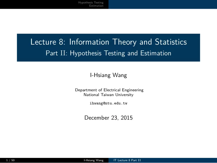
Hypothesis Testing Estimation Lecture 8: Information Theory and Statistics I-Hsiang Wang Department of Electrical Engineering National Taiwan University ihwang@ntu.edu.tw December 23, 2015 1 / 50 I-Hsiang Wang IT Lecture 8 Part II Part II : Hypothesis Testing and Estimation

Hypothesis Testing Estimation Basic Theory Asymptotics 1 Hypothesis Testing Basic Theory Asymptotics 2 Estimation Performance Evaluation of Estimators MLE, Asympototics, and Bayesian Estimators 2 / 50 I-Hsiang Wang IT Lecture 8 Part II

Hypothesis Testing Estimation Basic Theory Asymptotics 1 Hypothesis Testing Basic Theory Asymptotics 2 Estimation Performance Evaluation of Estimators MLE, Asympototics, and Bayesian Estimators 3 / 50 I-Hsiang Wang IT Lecture 8 Part II

Hypothesis Testing Estimation I-Hsiang Wang 4 / 50 Probability of miss detection (false negative; type II error): Probability of false alarm (false positive; type I error): 3 A popular measure of the cost is based on probability of errors: choose one of the two hypotheses, based on the observed realization IT Lecture 8 Part II We begin with the simplest setup – binary hypothesis testing: Basic Setup Asymptotics Basic Theory 1 Two hypotheses regarding the observation X , indexed by θ ∈ { 0 , 1 } : H 0 : X ∼ P 0 (Null Hypothesis, θ = 0 ) H 1 : X ∼ P 1 (Alternative Hypothesis, θ = 1 ) 2 Goal: design a decision making algorithm φ : X → { 0 , 1 } , x �→ ˆ θ , to of X , so that a certain cost (or risk ) is minimized. α φ ≡ P FA ( φ ) ≜ P {H 1 is chosen | H 0 } . β φ ≡ P MD ( φ ) ≜ P {H 0 is chosen | H 1 } .

Hypothesis Testing by its corresponding acceptance (decision) regions : I-Hsiang Wang 5 / 50 When the context is clear, we often drop the equivalently represented as Hence, the two types of probability of error can be Estimation IT Lecture 8 Part II Basic Theory Asymptotics Deterministic Testing Algorithm ≡ Decision Regions A test φ : X → { 0 , 1 } is equivalently characterized Observation Space A θ ( φ ) ≡ φ − 1 ( ) { } X ˆ x ∈ X : φ ( x ) = ˆ , ˆ ≜ θ θ θ = 0 , 1 . A 1 ( φ ) Acceptance Region of H 1 . ∑ P 0 ( x ) = ∑ α φ = φ ( x ) P 0 ( x ) , x ∈X x ∈A 1 ( φ ) ∑ P 1 ( x ) = ∑ (1 − φ ( x )) P 1 ( x ) . A 0 ( φ ) β φ = x ∈A 0 ( φ ) x ∈X Acceptance Region of H 0 . dependency on the test φ when dealing with acceptance regions A ˆ θ .

Hypothesis Testing Estimation I-Hsiang Wang 6 / 50 IT Lecture 8 Part II Definition 1 (Likelihood Ratio Test) Basic Theory Likelihood Ratio Test Asymptotics A (deteministic) likelihood ratio test (LRT) is a test φ τ , parametrized by constants τ > 0 (called threshold), defined as follows: { 1 if P 1 ( x ) > τ P 0 ( x ) φ τ ( x ) = if P 1 ( x ) ≤ τ P 0 ( x ) . 0 For x ∈ supp P 0 , the likelihood ratio L ( x ) ≜ P 1 ( x ) P 0 ( x ) . Hence, LRT is a thresholding algorithm on likelihood ratio L ( x ) . Remark : For computational convenience, often one deals with log likelihood ratio (LLR) log ( L ( x )) = log ( P 1 ( x )) − log ( P 0 ( x )) .

Hypothesis Testing Estimation I-Hsiang Wang 7 / 50 IT Lecture 8 Part II Theorem 1 (Neyman-Pearson Lemma) Basic Theory Asymptotics Trade-Off Between α (P FA ) and β (P MD ) For a likelihood ratio test φ τ and another deterministic test φ , α φ ≤ α φ τ = ⇒ β φ ≥ β φ τ . pf : Observe ∀ x ∈ X , 0 ≤ ( φ τ ( x ) − φ ( x )) ( P 1 ( x ) − τ P 0 ( x )) , because if P 1 ( x ) − τ P 0 ( x ) > 0 = ⇒ φ τ ( x ) = 1 = ⇒ ( φ τ ( x ) − φ ( x )) ≥ 0 . if P 1 ( x ) − τ P 0 ( x ) ≤ 0 = ⇒ φ τ ( x ) = 0 = ⇒ ( φ τ ( x ) − φ ( x )) ≤ 0 . Summing over all x ∈ X , we get 0 ≤ (1 − β φ τ ) − (1 − β φ ) − τ ( α φ τ − α φ ) = ( β φ − β φ τ ) + τ ( α φ − α φ τ ) . Since τ > 0 , from above we conclude that α φ ≤ α φ τ = ⇒ β φ ≥ β φ τ .

Hypothesis Testing Estimation I-Hsiang Wang 8 / 50 What is the optimal test achieving the curve? What is the optimal trade-off curve? Question : IT Lecture 8 Part II Basic Theory Asymptotics β ( P MD ) β ( P MD ) 1 1 α ( P FA ) α ( P FA ) 1 1

Hypothesis Testing Definition 3 (Randomized LRT) I-Hsiang Wang 9 / 50 Estimation IT Lecture 8 Part II Randomized tests include deterministic tests as special cases. Definition 2 (Randomized Test) Randomized Testing Algorithm Basic Theory Asymptotics A randomized test decides ˆ θ = 1 with probability φ ( x ) and ˆ θ = 0 with probability 1 − φ ( x ) , where φ is a mapping φ : X → [0 , 1] . Note : A randomized test is characterized by φ , as in deterministic tests. A randomized likelihood ratio test (LRT) is a test φ τ,γ , parametrized by cosntants τ > 0 and γ ∈ (0 , 1) , defined as follows:  1 if P 1 ( x ) > τ P 0 ( x )   φ τ,γ ( x ) = γ if P 1 ( x ) = τ P 0 ( x ) .   0 if P 1 ( x ) < τ P 0 ( x )

Hypothesis Testing Estimation I-Hsiang Wang 10 / 50 attains optimality for the Neyman-Pearson Problem . Theorem 2 (Neyman-Pearson) subject to IT Lecture 8 Part II minimize Neyman-Pearson Problem Consider the following optimization problem: Randomized LRT Achieves the Optimal Trade-Off Asymptotics Basic Theory β φ φ : X→ [0 , 1] α φ ≤ α ∗ A randomized LRT φ τ ∗ ,γ ∗ with the parameters ( τ ∗ , γ ∗ ) satisfying α ∗ = α φ τ ∗ ,γ ∗ ,

Hypothesis Testing Estimation I-Hsiang Wang 11 / 50 IT Lecture 8 Part II Basic Theory Asymptotics pf : First argue that for any α ∗ ∈ (0 , 1) , one can find ( τ ∗ , γ ∗ ) such that α ∗ = α φ τ ∗ ,γ ∗ = ∑ φ τ ∗ ,γ ∗ ( x ) P 0 ( x ) x ∈X ∑ ∑ x : L ( x )= τ ∗ γ ∗ P 0 ( x ) = x : L ( x ) >τ ∗ P 0 ( x ) + For any test φ , due to a similar argument as in Theorem 1, we have ∀ x ∈ X , ( φ τ ∗ ,γ ∗ ( x ) − φ ( x )) ( P 1 ( x ) − τ ∗ P 0 ( x )) ≥ 0 . Summing over all x ∈ X , similarly we get ( ) + τ ∗ ( ) β φ − β φ τ ∗ ,γ ∗ α φ − α φ τ ∗ ,γ ∗ ≥ 0 Hence, for any feasible test φ with α φ ≤ α ∗ = α φ τ ∗ ,γ ∗ , its probability of type II error β φ ≥ β φ τ ∗ ,γ ∗ .

Hypothesis Testing With prior probabilities, it then makes sense to talk about the average I-Hsiang Wang 12 / 50 error (or in general, a risk function) is minimized. with knowledge of prior probabilities so that the average probability of The Bayesian hypothesis testing problem is to test the two hypotheses Estimation IT Lecture 8 Part II Basic Theory Asymptotics Bayesian Setup Sometimes prior probabilities of the two hypotheses are known: π θ ≜ P {H θ is true } , θ = 0 , 1 , π 0 + π 1 = 1 . In this sense, one can view the index Θ as a (binary) random variable with (prior) distribution P { Θ = θ } = π θ , for θ = 0 , 1 . probability of error for a test φ , or more generally, the average cost (risk) : [ { }] Θ ̸ = ˆ P e ( φ ) ≜ π 0 α φ + π 1 β φ = E Θ , X Θ 1 , [ ] R ( φ ) ≜ E Θ , X . r Θ , ˆ Θ

Hypothesis Testing Estimation I-Hsiang Wang 13 / 50 attains optimality for the Bayesian Problem . threshold Theorem 3 (LRT is an Optimal Bayesian Test) with known IT Lecture 8 Part II Bayesian Problem Basic Theory Asymptotics Minimizing Bayes Risk minimize Consider the following problem of minimizing Bayes risk. [ ] R ( φ ) ≜ E Θ , X r Θ , ˆ Θ φ : X→ [0 , 1] ( π 0 , π 1 ) and r θ, ˆ θ Assume r 0 , 0 < r 0 , 1 and r 1 , 1 < r 1 , 0 . A deterministic LRT φ τ ∗ with τ ∗ = ( r 0 , 1 − r 0 , 0 ) π 0 ( r 1 , 0 − r 1 , 1 ) π 1

Hypothesis Testing Estimation I-Hsiang Wang 14 / 50 It is then obvious that we should choose IT Lecture 8 Part II Asymptotics Basic Theory pf : R ( φ ) = ∑ r 0 , 0 π 0 P 0 ( x ) (1 − φ ( x )) + ∑ r 0 , 1 π 0 P 0 ( x ) φ ( x ) x ∈X x ∈X + ∑ r 1 , 0 π 1 P 1 ( x ) (1 − φ ( x )) + ∑ r 1 , 1 π 1 P 1 ( x ) φ ( x ) x ∈X x ∈X = r 0 , 0 π 0 + ∑ ( r 0 , 1 − r 0 , 0 ) π 0 P 0 ( x ) φ ( x ) x ∈X + r 1 , 0 π 1 + ∑ ( r 1 , 1 − r 1 , 0 ) π 1 P 1 ( x ) φ ( x ) x ∈X ( ∗ ) � �� � [ ] = ∑ ( r 0 , 1 − r 0 , 0 ) π 0 P 0 ( x ) − ( r 1 , 1 − r 1 , 0 ) π 1 P 1 ( x ) φ ( x ) x ∈X + r 0 , 0 π 0 + r 1 , 0 π 1 . For each x ∈ X , we shall choose φ ( x ) ∈ [0 , 1] such that ( ∗ ) is minimized. { 1 if ( r 0 , 1 − r 0 , 0 ) π 0 P 0 ( x ) − ( r 1 , 1 − r 1 , 0 ) π 1 P 1 ( x ) < 0 φ ( x ) = if ( r 0 , 1 − r 0 , 0 ) π 0 P 0 ( x ) − ( r 1 , 1 − r 1 , 0 ) π 1 P 1 ( x ) ≥ 0 . 0

Hypothesis Testing Extensions include I-Hsiang Wang 15 / 50 with information theoretic tools. explore the asymptotic behavior of hypothesis testing, and the connection Here we do not pursue these directions further. Instead, we would like to Composite hypothesis testing, etc. Minimax risk optimization (with unknown prior) M -ary hypothesis testing and Neyman-Pearson settings. Estimation Moreover, a likelihood ratio test (LRT) is optimal both in the Bayesian turns out to be a sufficient statistics. For binary hypothesis testing problems, the likelihood ratio Discussions Asymptotics Basic Theory IT Lecture 8 Part II L ( x ) ≜ P 1 ( x ) P 0 ( x )

Hypothesis Testing Estimation Basic Theory Asymptotics 1 Hypothesis Testing Basic Theory Asymptotics 2 Estimation Performance Evaluation of Estimators MLE, Asympototics, and Bayesian Estimators 16 / 50 I-Hsiang Wang IT Lecture 8 Part II