From Maxent to Machine Learning and Back T. Sears ANU March 2007 - PowerPoint PPT Presentation
From Maxent to Machine Learning and Back T. Sears ANU March 2007 T. Sears (ANU) From Maxent to Machine Learning and Back Maxent 2007 1 / 36 50 Years Ago . . . The principles and mathematical methods of statistical mechanics are seen to
From Maxent to Machine Learning and Back T. Sears ANU March 2007 T. Sears (ANU) From Maxent to Machine Learning and Back Maxent 2007 1 / 36
50 Years Ago . . . ”The principles and mathematical methods of statistical mechanics are seen to be of much more general applicability. . . In the problem of prediction, the maximization of entropy is not an application of a law of physics, but merely a method of reasoning which ensures that no unconscious arbitrary assumptions have been introduced.” –E.T. Jaynes, 1957 T. Sears (ANU) From Maxent to Machine Learning and Back Maxent 2007 2 / 36
“. . . a method of reasoning . . . ” Jenkins, if I want another yes-man I’ll build one.
Outline Generalizing Maxent 1 Two Examples 2 Broader Comparisons 3 Extensions/Conclusions 4 T. Sears (ANU) From Maxent to Machine Learning and Back Maxent 2007 4 / 36
Generalizing Maxent You are here Generalizing Maxent 1 Two Examples 2 Broader Comparisons 3 Extensions/Conclusions 4 T. Sears (ANU) From Maxent to Machine Learning and Back Maxent 2007 5 / 36
Generalizing Maxent The Classic Maxent Problem Minimize negative entropy subject to linear constraints: A is M × N . N � M < N , a ”wide” matrix. min p S ( p ) := p i log( p i ) b is a data vector. i =1 � B � subject to A := T 1 Ap = b contains a normalization p i ≥ 0 constraint. T. Sears (ANU) From Maxent to Machine Learning and Back Maxent 2007 6 / 36
Generalizing Maxent Extending the Classic Maxent Problem min p S ( p ) subject to Ap = b Original problem. T. Sears (ANU) From Maxent to Machine Learning and Back Maxent 2007 7 / 36
Generalizing Maxent Extending the Classic Maxent Problem min p S ( p ) + δ { 0 } ( Ap − b ) Original problem. Convert constraints to a convex function. T. Sears (ANU) From Maxent to Machine Learning and Back Maxent 2007 7 / 36
Generalizing Maxent Extending the Classic Maxent Problem min p S ( p ) + δ { 0 } ( || Ap − b || P ) Original problem. Convert constraints to a convex function. Use any norm... T. Sears (ANU) From Maxent to Machine Learning and Back Maxent 2007 7 / 36
Generalizing Maxent Extending the Classic Maxent Problem min p S ( p ) + δ ǫ B P ( Ap − b ) Original problem. Convert constraints to a convex function. Use any norm... and relax constraints. T. Sears (ANU) From Maxent to Machine Learning and Back Maxent 2007 7 / 36
Generalizing Maxent Extending the Classic Maxent Problem min p ∆ F ( p , p 0 ) + δ ǫ B P ( Ap − b ) Original problem. Convert constraints to a convex function. Use any norm... and relax constraints. Generalize SBG entropy to Bregman divergence. T. Sears (ANU) From Maxent to Machine Learning and Back Maxent 2007 7 / 36
Generalizing Maxent Extending the Classic Maxent Problem µ F ∗ ( A T µ + p ∗ min 0 ) + � µ , b � + ǫ || µ || Q Original problem. Convert constraints to a convex function. Use any norm... and relax constraints. Generalize SBG entropy to Bregman divergence. Find the Fenchel dual problem to solve. T. Sears (ANU) From Maxent to Machine Learning and Back Maxent 2007 7 / 36
Generalizing Maxent Extending the Classic Maxent Problem µ F ∗ ( A T µ + p ∗ min 0 ) + � µ , b � + ǫ || µ || Q � �� � � �� � ”Likelihood” ”Prior” Original problem. Convert constraints to a convex function. Use any norm... and relax constraints. Generalize SBG entropy to Bregman divergence. Find the Fenchel dual problem to solve. It’s a more general form of the MAP problem. T. Sears (ANU) From Maxent to Machine Learning and Back Maxent 2007 7 / 36
Generalizing Maxent Characterizing the solution Compare to statistical models After solving for ¯ µ we can recover the optimal primal solution: ”Score” ���� A T ¯ p = ∇ F ∗ µ + p ∗ ¯ ( 0 ) ���� ”Family” T. Sears (ANU) From Maxent to Machine Learning and Back Maxent 2007 8 / 36
Generalizing Maxent Characterizing the solution Compare to statistical models After solving for ¯ µ we can recover the optimal primal solution: ”Score” ���� A T ¯ p = ∇ F ∗ µ + p ∗ ¯ ( 0 ) ���� ”Family” p comes from a family of distributions. ¯ T. Sears (ANU) From Maxent to Machine Learning and Back Maxent 2007 8 / 36
Generalizing Maxent Characterizing the solution Compare to statistical models After solving for ¯ µ we can recover the optimal primal solution: ”Score” ���� A T ¯ p = ∇ F ∗ µ + p ∗ ¯ ( 0 ) ���� ”Family” p comes from a family of distributions. ¯ Entropy function ( F ) determines the family ( ∇ F ∗ ). T. Sears (ANU) From Maxent to Machine Learning and Back Maxent 2007 8 / 36
Generalizing Maxent Characterizing the solution Compare to statistical models After solving for ¯ µ we can recover the optimal primal solution: ”Score” ���� A T ¯ p = ∇ F ∗ µ + p ∗ ¯ ( 0 ) ���� ”Family” p comes from a family of distributions. ¯ Entropy function ( F ) determines the family ( ∇ F ∗ ). SBG entropy → exponential family. T. Sears (ANU) From Maxent to Machine Learning and Back Maxent 2007 8 / 36
Generalizing Maxent Characterizing the solution Compare to statistical models After solving for ¯ µ we can recover the optimal primal solution: ”Score” ���� A T ¯ p = ∇ F ∗ µ + p ∗ ¯ ( 0 ) ���� ”Family” p comes from a family of distributions. ¯ Entropy function ( F ) determines the family ( ∇ F ∗ ). SBG entropy → exponential family. Any “nice” F → some family. T. Sears (ANU) From Maxent to Machine Learning and Back Maxent 2007 8 / 36
Generalizing Maxent Generalizing the Exponential Family q-Exponential exp q 8 q � 1.5 6 q � 1. 4 q � 0.5 2 Asymptote for q � 1.5 � 3 � 2 � 1 0 1 2 3 1 1 − q (1 + (1 − q ) p ) q � = 1 + exp q ( p ) := exp( p ) q = 1 T. Sears (ANU) From Maxent to Machine Learning and Back Maxent 2007 9 / 36
Generalizing Maxent Tail Behavior Tail Behavior exp q 1.0 0.8 0.6 0.4 0.2 � 3.0 � 2.5 � 2.0 � 1.5 � 1.0 � 0.5 0.0 q > 1 naturally gives fat tails. q < 1 truncates the tail. T. Sears (ANU) From Maxent to Machine Learning and Back Maxent 2007 10 / 36
Two Examples You are here Generalizing Maxent 1 Two Examples 2 Broader Comparisons 3 Extensions/Conclusions 4 T. Sears (ANU) From Maxent to Machine Learning and Back Maxent 2007 11 / 36
Two Examples Loaded Die Example Setup A die with 6 faces. T. Sears (ANU) From Maxent to Machine Learning and Back Maxent 2007 12 / 36
Two Examples Loaded Die Example Setup A die with 6 faces. Expected value of 4.5, instead of 3.5 for a “fair die”. T. Sears (ANU) From Maxent to Machine Learning and Back Maxent 2007 12 / 36
Two Examples Loaded Die Example Setup A die with 6 faces. Expected value of 4.5, instead of 3.5 for a “fair die”. For this problem: � 1 � 4 . 5 � � 2 3 4 5 6 A = and b = 1 1 1 1 1 1 1 T. Sears (ANU) From Maxent to Machine Learning and Back Maxent 2007 12 / 36
Two Examples Loaded Die Example Setup A die with 6 faces. Expected value of 4.5, instead of 3.5 for a “fair die”. For this problem: � 1 � 4 . 5 � � 2 3 4 5 6 A = and b = 1 1 1 1 1 1 1 Find p , assuming S → S q , p 0 is uniform, ǫ = 0. T. Sears (ANU) From Maxent to Machine Learning and Back Maxent 2007 12 / 36
Two Examples Loaded Die Example Setup A die with 6 faces. Expected value of 4.5, instead of 3.5 for a “fair die”. For this problem: � 1 � 4 . 5 � � 2 3 4 5 6 A = and b = 1 1 1 1 1 1 1 Find p , assuming S → S q , p 0 is uniform, ǫ = 0. T. Sears (ANU) From Maxent to Machine Learning and Back Maxent 2007 12 / 36
Two Examples Loaded Die Example Setup A die with 6 faces. Expected value of 4.5, instead of 3.5 for a “fair die”. For this problem: � 1 � 4 . 5 � � 2 3 4 5 6 A = and b = 1 1 1 1 1 1 1 Find p , assuming S → S q , p 0 is uniform, ǫ = 0. T. Sears (ANU) From Maxent to Machine Learning and Back Maxent 2007 12 / 36
Two Examples Loaded Die Example Probability q � Sensitivity of Each Event Varies q 0.3 0.1 1. 1.9 0.2 0.1 0.0 Higher q raises weight on face 1 and face 6. Opposite for 3,4,5. Task: Make a two-way market on each die face. Which is easiest? T. Sears (ANU) From Maxent to Machine Learning and Back Maxent 2007 13 / 36
Two Examples Example: The Dantzig Selector Entropy Function as Prior Information Background: Consider a variation on linear regression � y = X β . Choose β via β || β || 1 + δ ǫ B ∞ ( X T ( X β − y )) min T. Sears (ANU) From Maxent to Machine Learning and Back Maxent 2007 14 / 36
Two Examples Example: The Dantzig Selector Entropy Function as Prior Information Background: Consider a variation on linear regression � y = X β . Choose β via β || β || 1 + δ ǫ B ∞ ( X T ( X β − y )) min The non-zero entries of the solution can exactly identify the correct set of regressors with high probability under special conditions. (Candace and Tao, Ann. Stat. 2007) T. Sears (ANU) From Maxent to Machine Learning and Back Maxent 2007 14 / 36
Recommend
More recommend
Explore More Topics
Stay informed with curated content and fresh updates.
