Lecture 8: Fitting Tuesday, Sept 25 Announcements, schedule Grad - PDF document
Lecture 8: Fitting Tuesday, Sept 25 Announcements, schedule Grad student extensions Due end of term Data sets, suggestions Reminder: Midterm Tuesday 10/9 Problem set 2 out Thursday, due 10/11 Outline Review from
Lecture 8: Fitting Tuesday, Sept 25
Announcements, schedule • Grad student extensions – Due end of term – Data sets, suggestions • Reminder: Midterm Tuesday 10/9 • Problem set 2 out Thursday, due 10/11
Outline • Review from Thursday (affinity, cuts) • Local scale and affinity computation • Hough transform • Generalized Hough transform – Shape matching applications • Fitting lines – Least squares – Incremental fitting, k-means
Real Modality Analysis Tessellate the space Run the procedure in parallel with windows
Real Modality Analysis The blue data points were traversed by the windows towards the mode Slide by Y. Ukrainitz & B. Sarel
Mean shift • Labeling of data points: points visited by any window converging to same mode get the same label • [Comaniciu & Meer, PAMI 2002] : If data point is visited by multiple diverging mean shift processes, “majority vote”
Weighted graph representation (“Affinity matrix”)
Images as graphs q C pq c p Fully-connected graph • node for every pixel • link between every pair of pixels, p , q • similarity c pq for each link » similarity is inversely proportional to difference in color and position Slide by Steve Seitz
Segmentation by Graph Cuts w A B C Break Graph into Segments • Delete links that cross between segments • Easiest to break links that have low similarity – similar pixels should be in the same segments – dissimilar pixels should be in different segments
Example Dimension of points : d = 2 Number of points : N = 4
Distance matrix D(:,1)= 0.01 D(1,:)= (0) 0.24 0.01 0.47 0.24 0.47 for i=1:N for j=1:N D(i,j) = ||x i - x j || 2 end end
Distance matrix D(:,1)= D(1,:)= (0) 0.24 0.01 0.47 0.29 0.24 (0) 0.29 0.15 0.24 0.15 for i=1:N for j=1:N D(i,j) = ||x i - x j || 2 end end
Distance matrix N x N matrix for i=1:N for j=1:N D(i,j) = ||x i - x j || 2 end end
Measuring affinity • One possibility: • Map distances to similarities, use as edge weights on graph
Distances � affinities D A for i=1:N for i=1:N for j=1:N for j=1:N D(i,j) = ||x i - x j || 2 A(i,j) = exp(-1/(2* σ ^2)*||x i - x j || 2 ) end end end end
Measuring affinity • One possibility: • Essentially, affinity drops off after distance gets past some threshold Small sigma: group Large sigma: only nearby points group distant Increasing sigma points
Scale affects affinity D=
Shuffling the affinity matrix • Permute the order of the vertices, in terms of how they are associated with the matrix rows/cols
Scale affects affinity Points x 1 …x 10 σ =.2 Data points Points x 31 …x 40 σ =.1 σ =.2 σ =1 Affinity matrices
Eigenvectors and graph cuts w’ A w w’Aw = ΣΣ w i A ij w j i j
Eigenvectors and graph cuts • Want a vector w giving the “association” between each element and a cluster • Want elements within this cluster to have strong affinity with one another a T Aa w w • Maximize subject to the constraint a T a = 1 w w . . . Aw = λ w Eigenvalue problem : choose the eigenvector of A with largest eigenvalue
Rayleigh Quotient
Example Data points Affinity matrix eigenvector
Eigenvectors and multiple cuts • Use eigenvectors associated with k largest eigenvalues as cluster weights • Or re-solve recursively
Scale affects affinity, number of clusters Multi- scale data Scale really affects clusters [Self-Tuning Spectral Clustering, L. Zelnik-Manor and P. Perona, NIPS 2004]
Local scale selection • Possible solution: choose sigma per point Distance to Kth neighbor for point s_i [Self-Tuning Spectral Clustering, L. Zelnik-Manor and P. Perona, NIPS 2004]
Local scale selection [Self-Tuning Spectral Clustering, L. Zelnik-Manor and P. Perona, NIPS 2004]
Local scale selection, synthetic data [Self-Tuning Spectral Clustering, L. Zelnik-Manor and P. Perona, NIPS 2004]
Local scale selection, image data Image segmentation results, based on gray-scale differences alone. The number of clusters was set manually here to force a large number of clusters. Since the scale is tuned locally for each pixel we obtained segments with both high and low contrast to the surrounding. Zelnik-Manor & Perona, http://www.vision.caltech.edu/lihi/Demos/SelfTuningClustering.html
Fitting • Want to associate a model with observed features [Fig from Marszalek & Schmid, 2007]
Fitting lines • Given points that belong to a line, what is the line? • How many lines are there? • Which points belong to which lines?
Difficulty of fitting lines • Extraneous data: clutter, multiple models • Missing data: only some parts of model are present • Noise in the measured edge points, orientations …Enter: • Cost: infeasible to check all Voting combinations of features by schemes fitting a model to each possible subset
Hough transform • Maps model (pattern) detection problem to simple peak detection problem • Record all the structures on which each point lies, then look for structures that get many votes • Useful for line fitting
Finding lines in an image y b b 0 m 0 x m image space Hough (parameter) space Connection between image (x,y) and Hough (m,b) spaces • A line in the image corresponds to a point in Hough space • To go from image space to Hough space: – given a set of points (x,y), find all (m,b) such that y = mx + b Slide credit: Steve Seitz
Finding lines in an image y b y 0 x 0 x m image space Hough (parameter) space Connection between image (x,y) and Hough (m,b) spaces • A line in the image corresponds to a point in Hough space • To go from image space to Hough space: – given a set of points (x,y), find all (m,b) such that y = mx + b • What does a point (x 0 , y 0 ) in the image space map to? – Answer: the solutions of b = -x 0 m + y 0 – this is a line in Hough space
Finding lines in an image y b y 0 x 0 x m image space Hough (parameter) space Connection between image (x,y) and Hough (m,b) spaces • A line in the image corresponds to a point in Hough space • To go from image space to Hough space: – given a set of points (x,y), find all (m,b) such that y = mx + b • What does a point (x 0 , y 0 ) in the image space map to? – Answer: the solutions of b = -x 0 m + y 0 – this is a line in Hough space
Polar representation for lines • Issues with ( m , b ) parameter space: – Can take on infinite values – Undefined for vertical lines (x=constant)
Polar representation for lines x [0,0] ө d : perpendicular distance d from line to origin y ө : angle the perpendicular makes with the x-axis (0 <= ө <= 2 π ) x cos ө + y sin ө + d = 0 Point in image space � sinusoid segment in Hough space
Hough transform algorithm Using the polar parameterization: H: accumulator array (votes) θ Basic Hough transform algorithm 1. Initialize H[d, θ ]=0 2. for each edge point I[x,y] in the image for θ = 0 to 180 // some quantization d H[d, θ ] += 1 3. Find the value(s) of (d, θ ) where H[d, θ ] is maximum 4. The detected line in the image is given by Hough line demo Time complexity (in terms of number of votes)?
Example: Hough transform for straight lines d y θ x Image space Votes edge coordinates
Example: Hough transform for straight lines Square : Circle :
Example: Hough transform for straight lines
Example with noise d y x θ Image space Votes edge coordinates
Example with noise / random points Image space Votes edge coordinates
Extensions Extension 1: Use the image gradient 1. same 2. for each edge point I[x,y] in the image compute unique (d, θ ) based on image gradient at (x,y) H[d, θ ] += 1 3. same 4. same (Reduces degrees of freedom) Extension 2 • give more votes for stronger edges Extension 3 change the sampling of (d, θ ) to give more/less resolution • Extension 4 • The same procedure can be used with circles, squares, or any other shape
Recall: Image gradient The gradient of an image: The gradient points in the direction of most rapid change in intensity The gradient direction (orientation of edge normal) is given by: The edge strength is given by the gradient magnitude
Extensions Extension 1: Use the image gradient 1. same 2. for each edge point I[x,y] in the image compute unique (d, θ ) based on image gradient at (x,y) H[d, θ ] += 1 3. same 4. same (Reduces degrees of freedom) Extension 2 • give more votes for stronger edges (use magnitude of gradient) Extension 3 change the sampling of (d, θ ) to give more/less resolution • Extension 4 • The same procedure can be used with circles, squares, or any other shape…
Hough transform for circles • Circle: center (a,b) and radius r − + − = 2 2 2 ( x a ) ( y b ) r i i • For a fixed radius r, unknown gradient direction Hough space Image space
Hough transform for circles • Circle: center (a,b) and radius r − + − = 2 2 2 ( x a ) ( y b ) r i i • For unknown radius r, unknown gradient direction Image space Hough space
Recommend
More recommend
Explore More Topics
Stay informed with curated content and fresh updates.
