Lecture 5: Sampling (Monte Carlo Methods) Julia Hockenmaier - PowerPoint PPT Presentation
CS598JHM: Advanced NLP (Spring 2013) http://courses.engr.illinois.edu/cs598jhm/ Lecture 5: Sampling (Monte Carlo Methods) Julia Hockenmaier juliahmr@illinois.edu 3324 Siebel Center Office hours: by appointment The goal of Monte Carlo
CS598JHM: Advanced NLP (Spring 2013) http://courses.engr.illinois.edu/cs598jhm/ Lecture 5: Sampling (Monte Carlo Methods) Julia Hockenmaier juliahmr@illinois.edu 3324 Siebel Center Office hours: by appointment
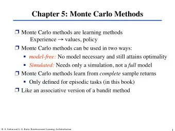
The goal of Monte Carlo methods Given a target distribution P( x ) that we cannot evaluate exactly, we use Monte Carlo (= sampling) methods to: 1. Generate samples { x (1) ... x (r) ... x (R) } from P( x ) 2. Estimate the expectation of functions φ ( x ) under P( x ) In Bayesian approaches, model parameters θ are also random variables. So, the target distribution P( x ) may in fact be P( θ | D ), the posterior of θ given the data 2 Bayesian Methods in NLP
The expectation Φ of φ ( x ): Φ = 〈φ ( x ) 〉 P( x ) = ∑ x P( x ) φ ( x ) We can estimate Φ by Monte Carlo integration: Draw a finite number of samples { x (1) ... x (R) } from P( x ) and estimate Φ as Φ = 1 ˆ X φ ( x ( r ) ) R r The variance of Φ is a function of σ 2 / R ( σ 2 is the variance of φ ( x ); R is the number of samples). σ 2 = E[( φ − Φ ) 2 | x ] = ∑ x P( x ) ( φ ( x ) − Φ ) 2 The accuracy of Φ is independent of the dimensionality of x . A dozen independent samples from P( x ) may be enough 3 Bayesian Methods in NLP
Why is sampling hard? We need to be able to draw independent samples from P( x ) This is difficult, because: - Our models are often of the form P( x ) ∝ f( x ) i.e P( x ) = f( x ) / Z - We often cannot compute the partition function Z = ∑ x’ f( x’ ) because we usually operate in very high dimensions (or very large state spaces). 4 Bayesian Methods in NLP
Sampling methods Sampling from a fixed proposal distribution Q( x ) ≠ P( x ): - Uniform sampling - Importance sampling - Rejection sampling Markov Chain Monte Carlo (MCMC) Sampling from a Markov chain: the probability of the next sample (= proposal distribution) depends on the current state - Metropolis-Hastings - Gibbs sampling 5 Bayesian Methods in NLP
Uniform sampling Assume Q( x ) is uniform. Draw samples x (r) ∼ Q( x ) (uniformly) from the state space, evaluate P( x (r) ) at x (r) This gives a new distribution f ( x ( r ) ) P 0 ( x ( r ) ) = P R i =1 f ( x ( i ) ) Estimate 〈 φ ( x ) 〉 P( x ) as ˆ X φ ( x ( r ) ) P 0 ( x ( r ) ) Φ = r Problem: Unless P( x ) itself is close to uniform, this strategy will be very inefficient. In high-dimensional spaces, most regions of the state space have typically very low probability 6 Bayesian Methods in NLP
Importance sampling Importance sampling can be used to compute expectations Φ f( x ) g( x ) Assumptions: - We can evaluate P( x ) ∝ f( x ) at any point - We have a simple sample density Q( x ) ∝ g( x ), which we can evaluate and draw samples from, - For any x: if P( x ) > 0, then also Q( x ) > 0 Algorithm - Draw samples from Q( x ) ∝ g( x ) - Re-weight samples by w r = f( x (r) )/g( x (r) ) - Estimate Φ as Φ = ∑ r w r φ ( x ( r ) ) ˆ ∑ r w r This converges to Φ . But: We can’t estimate the variance of Φ . The empirical variances of w r and w r φ ( x (r) ) may not be a good indicator of their true variances 7 Bayesian Methods in NLP
Rejection sampling Assumptions: - We can evaluate P( x ) ∝ f( x ) at any point - We have a simple proposal density Q( x ) ∝ g( x ), which we can evaluate and draw samples from - We know the value of a constant c such that c g( x ) > f( x ) f( x ) c g(x’) Algorithm : c g( x ) c g(x) - Sample x ∼ Q( x ) and evaluate c g( x ) - Sample y ∼ Uniform([0, c g( x )]) y’ reject x ! accept y - If f( x ) ≥ y , accept x , else reject x x ! x x’ This returns independent samples from P( x ) Problems: Acceptance rate: ∫ P( x )d x / ∫ c Q( x ) d x = 1/ c But c grows exponentially with the dimensionality of x 8 Bayesian Methods in NLP
Markov Chain Monte Carlo f( x ) Rejection sampling and importance sampling Q( x;x (1) ) only work well when Q( x ) is similar to P( x ). x (1) This is difficult to achieve in high dimensions. ... f( x ) Markov Chain Monte Carlo methods generate Q( x;x (25) ) a sequence of samples x (1)... x (t)... x (T) x (25) ... x (t+1) is drawn from a proposal distribution Q( x ; x (t) ) which depends on the last sample x (t) Advantage : Q( x ; x (t) ) does not have to be similar to P( x ) Disadvantage : the samples x (t) are correlated, and not independent. We may have to generate a lot of samples ( T ≫ R) to get a sequence of R independent samples x (1)... x (R) 9 Bayesian Methods in NLP
Markov chains A (discrete-time, discrete-state) Markov chain over N states {x 1 ,...,x N } is defined by - an N- dimensional multinomial P (0) , the initial distribution over the states {x 1 ,...,x N } - an N × N transition matrix A that defines the transition probability of moving from state x i to state x j : A ij = P(X (t+1) = x j | X (t) = x i ) The Markov chain defines a sequence of distributions P (0) ...P (t) ... over the states {x 1 ,...,x N }: P (t) = P (t -1) × A = P (0) × A (t-1) 10 Bayesian Methods in NLP
More Markov chain terminology A Markov chain is irreducible if any state can be reached from any other state with nonzero probability. An irreducible Markov chain is recurrent if the probability of reaching any state x j from any state x i in finite time is 1. An irreducible, recurrent Markov chain is positive recurrent if it has a stationary (= equilibrium) distribution π = lim t →∞ P (t) An ergodic Markov chain will converge to π regardless of its start state. A reversible Markov chain obeys detailed balance: π (x i ) P(X (t+1) = x j | X (t) = x i ) = π (x j ) P(X (t+1) = x i | X (t) = x j ) 11 Bayesian Methods in NLP
MCMC: Metropolis-Hastings Algorithm: 1. Given the last sample x (t) , generate x ’ ∼ Q( x ; x (t) ) Q ( x ( t ) ; x 0 ) Q ( x ( t ) ; x 0 ) a = f ( x 0 ) Q ( x 0 ; x ( t ) ) = P ( x 0 ) 2. Compute f ( x ( t ) ) P ( x ( t ) ) Q ( x 0 ; x ( t ) ) 3. If a > 1: accept x ` Otherwise, accept x ` with probability a 4. If x ’ is accepted: x (t+1) = x ` Otherwise, x (t+1) = x (t) Regardless of Q( x ; x (t) ), this algorithm samples from an ergodic Markov chain with states x and stationary distribution P( X ). 12 Bayesian Methods in NLP
Why Q(x; x (t) ) can be any distribution = f ( x j ) Q ( x i ; x j ) = P ( x j ) Q ( x i ; x j ) Q ( x i ; x j ) Q ( x i ; x j ) = 1 a ij f ( x i ) P ( x i ) a ji accept ( x i , x j ) = min ( 1 , a ij ) accept ( x i , x j ) < 1 ⇒ accept ( x j , x i ) = 1 The transition matrix of the Markov chain is defined as P ( x j | x i ) = Q ( x j ; x i ) accept ( x i , x j ) x i � Z P ( x j | x i ) = Q ( x j ; x i )+ Q ( x k ; x i ) accept ( x i , x k ) 1 � d x k x i Assume accept( x i , x j ) = a ij < 1. Thus accept( x j , x i ) = 1 accept( x i , x j ) P ( x i ) Q ( x j ; x i ) = P ( x j ) Q ( x i ; x j ) accept( x j , x i ) P ( x i ) P ( x j | x i ) = P ( x j ) P ( x i | x j ) This obeys detailed balance. The equilibrium distribution is P ( x i ) regardless of Q ( x ’; x ) 13 Bayesian Methods in NLP
Why Q(x; x (t) ) still matters Convergence: How many steps does it take to reach the equilibrium distribution? - If Q is positive ( Q( x’; x ) > 0 for all x’; x ), the distribution of x (t) is guaranteed to converge to P( x ) in the limit. - But: convergence is difficult to assess. - The steps before equilibrium is reached should be ignored ( burn-in) Mixing: How fast does the chain move around the state space? Rejection rate: - If the step size (distance btw. x ’ and x (t) ) is large, the rejection probability can be high - If the step size is too small, only a small region of the sample space may be explored (= slow mixing) 14 Bayesian Methods in NLP
MCMC variants Metropolis algorithm Q( x’; x ) is symmetric: Q( x’; x ) = Q( x; x’ ) a = f ( x 0 ) f ( x ( t ) ) = P ( x 0 ) P ( x ( t ) ) Single-component Metropolis-Hastings - x is divided into components x 1 ... x n Notation: x - i := { x 1 , ..., x i-1 , x i+1 , ..., x n } ( all components other than x i ) - At each iteration t , sample each x i in turn, using the full conditional distribution P ( x i | x - i ) = P ( x )/ ∫ P ( x ) d x i and proposal distributions Q i ( x i | x i(t) , x - i(t) ) and Q i ( x i(t) | x i , x - i(t) ) 15 Bayesian Methods in NLP
MCMC: Gibbs sampling Assumptions: - x is a multivariate random variable: x = (x 1 ,...,x n ) - The full conditionals P(x i | x 1 ,...,x i-1, x i+1 ,...,x n ) (=the conditional probabilities of each component given the rest) , are easy to evaluate (also true if we split the components of x into blocks) Algorithm: for t = 1...T: for i = 1...N: sample x i(t) ∼ P ( x i | x 1(t) ,..., x i-1(t), x i+1(t-1) ,..., x n(t-1) ) Gibbs sampling is single-component Metropolis-Hastings without rejection. Think of it as using the full conditionals as proposal distributions (so the two fractions cancel, and hence a = 1 ) Q i ( x i | x i(t) , x - i(t) ) = P ( x i | x 1(t) ,..., x i-1(t), x i+1(t-1) ,..., x n(t-1) ) Q i ( x i(t) | x i , x - i(t) ) = P ( x i(t) | x 1(t) ,..., x i-1(t), x i+1(t-1) ,..., x n(t-1) ) 16 Bayesian Methods in NLP
Recommend
More recommend
Explore More Topics
Stay informed with curated content and fresh updates.

