Lecture 22 Interpolation, Overfitting, Ridgeless Regression, and - PowerPoint PPT Presentation
Lecture 22 Interpolation, Overfitting, Ridgeless Regression, and Neural Networks Sasha Rakhlin Nov 21, 2019 1 / 32 In the previous lecture, we derived upper bounds on Rademacher averages of a set of neural networks in terms of norms of weight
Lecture 22 Interpolation, Overfitting, Ridgeless Regression, and Neural Networks Sasha Rakhlin Nov 21, 2019 1 / 32
In the previous lecture, we derived upper bounds on Rademacher averages of a set of neural networks in terms of norms of weight matrices, without explicit dependence on the number of neurons. Such a result is useful to control uniform deviations between empirical and expected errors, or for margin-based bounds. As we discussed earlier, analyses that employ uniform deviations are not the only path to understanding the out-of-sample performance. Today we will discuss methods for which empirical fit can be zero while out-of-sample is far from zero. In such situations, the bias-variance decomposition (rather than the estimation-approximation decomposition) might be more useful. 2 / 32
Bias-Variance Bias-Variance decomposition: f n − E Y 1 ∶ n [̂ 2 + E ∥ E Y 1 ∶ n [̂ 2 = E ∥̂ f n ]∥ f n ] − f ∗ ∥ 2 . E ∥̂ f n − f ∗ ∥ Recall that the above estimation error can be written as prediction error: E ∥̂ 2 = E (̂ f n − f ∗ ∥ f n ( X ) − Y ) 2 − min E ( f ( X ) − Y ) 2 f 3 / 32
Outline Local Kernel Regression: Nadaraya-Watson Interpolation Local Methods Kernel Ridge(less) Regression Wide Neural Networks Summary 4 / 32
Nadaraya-Watson estimator: ̂ f n ( x ) = n Y i W i ( x ) ∑ i = 1 with K h ( x − X i ) W i ( x ) = i = 1 K h ( x − X i ) ∑ n Here K h ( x − X i ) is a notion of “distance” between x and X i . 5 / 32
Fix a kernel K ∶ R d → R ≥ 0 . Assume K is zero outside unit Euclidean ball at origin (not true for e − x 2 , but close enough). (figure from Gy¨ orfi et al) Let K h ( x ) = K ( x / h ) , and so K h ( x − x ′ ) is zero if ∥ x − x ′ ∥ ≥ h . h is “bandwidth” – tunable parameter. Assume K ( x ) > c I {∥ x ∥ ≤ 1 } for some c > 0. This is important for the “averaging effect” to kick in. 6 / 32
Unlike the k-NN example, bias is easier to estimate. Bias: for a given x , E Y 1 ∶ n [̂ f n ( x )] = E Y 1 ∶ n [ n Y i W i ( x )] = n f ∗ ( X i ) W i ( x ) ∑ ∑ i = 1 i = 1 and so E Y 1 ∶ n [̂ f n ( x )] − f ∗ ( x ) = ( f ∗ ( X i ) − f ∗ ( x )) W i ( x ) n ∑ i = 1 Suppose f ∗ is 1-Lipschitz. Since K h is zero outside the h -radius ball, ∣ E Y 1 ∶ n [̂ f n ( x )] − f ∗ ( x )∣ 2 ≤ h 2 . 7 / 32
Variance: we have f n ( x ) − E Y 1 ∶ n [̂ ̂ f n ( x )] = n ( Y i − f ∗ ( X i )) W i ( x ) ∑ i = 1 Expectation of square of this difference is at most E [ n ( Y i − f ∗ ( X i )) 2 W i ( x ) 2 ] ∑ i = 1 since cross terms are zero (fix X ’s, take expectation with respect to the Y ’s). We are left analyzing K h ( x − X 1 ) 2 n E [ i = 1 K h ( x − X i )) 2 ] ( ∑ n Under some assumptions on density of X , the denominator is at least ( nh d ) 2 with high prob, whereas E K h ( x − X 1 ) 2 = O ( h d ) assuming ∫ K 2 < ∞ . This gives an overall variance of O ( 1 /( nh d )) . Many details skipped here (e.g. problems at the boundary, assumptions, etc) 8 / 32
1 Overall, bias and variance with h ∼ n − 2 + d yield 2 ≲ h 2 + 1 E ∥̂ 2 f n − f ∗ ∥ nh d = n − 2 + d 9 / 32
Outline Local Kernel Regression: Nadaraya-Watson Interpolation Local Methods Kernel Ridge(less) Regression Wide Neural Networks Summary 10 / 32
Can a learning method be successful if it interpolates the training data? 11 / 32
Bias-Variance and Overfitting “Elements of Statistical Learning,” Hastie, Tibshirani, Friedman 12 / 32
Outline Local Kernel Regression: Nadaraya-Watson Interpolation Local Methods Kernel Ridge(less) Regression Wide Neural Networks Summary 13 / 32
Consider the Nadaraya-Watson estimator. Take a kernel that approaches a large value τ at 0, e.g. K ( x ) = min { 1 / ∥ x ∥ α , τ } Large τ means ̂ f n ( X i ) ≈ Y i since the weight W i ( X i ) is dominating. If τ = ∞ , we get interpolation ̂ f n ( X i ) = Y i of all training data. Yet, the sketched proof still goes through. Hence, “memorizing the data” (governed by parameter τ ) is completely decoupled from the bias-variance trade-off (as given by parameter h ). Contrast with conventional wisdom: fitting data too well means overfitting. NB: Of course, we could always redefine any ̂ f n to be equal to Y i on X i , but our example shows more explicitly how memorization is governed by a parameter that is independent of bias-variance. 14 / 32
What is overfitting ? ▸ Fitting data too well? ▸ Bias too low, variance too high? Key takeaway: we should not conflate these two. 15 / 32
Outline Local Kernel Regression: Nadaraya-Watson Interpolation Local Methods Kernel Ridge(less) Regression Wide Neural Networks Summary 16 / 32
We saw that local methods such as Nadaraya-Watson can interpolate the data yet generalize. How about global methods such as (regularized) least squares? Below, we will show that minimum-norm interpolants of the data (which can be seen as limiting solutions when we turn off regularization) can indeed generalize. 17 / 32
First, recall Ridge Regression ̂ (⟨ w , x i ⟩ − y i ) 2 + λ ∥ w ∥ 2 n w λ = argmin ∑ w ∈ R d i = 1 has closed-form solution T ( XX ̂ T + λI ) − 1 Y n w λ = X = X T c = ∑ c i x i �ÜÜÜÜÜÜÜÜÜÜÜÜÜÜÜÜÜÜÜÜÜÜÜÜÜÜÜÜÜÜÜÜÜÜÜÜÜ�ÜÜÜÜÜÜÜÜÜÜÜÜÜÜÜÜÜÜÜÜÜÜÜÜÜÜÜÜÜÜÜÜÜÜÜÜÜ� i = 1 c implying functional form f λ ( x ) = ⟨̂ w λ , x ⟩ = n c i ⟨ x , x i ⟩ ˆ ∑ i = 1 18 / 32
Kernel Ridge Regression: n ( f ( x i ) − y i ) 2 + λ ∥ f ∥ 2 f λ = argmin ˆ ∑ K f ∈F i = 1 Representer Theorem: n f λ ( x ) = ˆ ∑ c i K ( x , x i ) (1) i = 1 Solution to Kernel Ridge Regression is given by [ K ] i , j = K ( x i , x j ) . c = ( K + λI ) − 1 Y , and functional form (1) can be written succinctly as f λ ( x ) = K ( x , X ) T ( K + λI ) − 1 Y ˆ where K ( x , X ) = [ K ( x , x 1 ) , K ( x , x 2 ) , . . . , K ( x , x n )] T . 19 / 32
Min-Norm Interpolation ( Ridgeless Regression) Linear case with n < d : the limiting solution λ → 0 is the minimum norm solution that interpolates the data. Indeed, w 0 = X ̂ T ( XX T ) − 1 Y is the unique solution in the span of the data. Solutions outside the span have larger norms. Kernel case: λ → 0 solution (as a function) is ˆ f 0 ( x ) = K ( x , X ) T K − 1 Y which we can write as solution to ∥ f ∥ K argmin f ∈F f ( x i ) = y i s.t. 20 / 32
Bias-Variance Analysis of Kernel Ridgeless Regression Variance: we have ̂ f n ( x ) − E Y 1 ∶ n [̂ f n ( x )] = K ( x , X ) T K − 1 ( Y − f ∗ ( X )) where f ∗ ( X ) = [ f ∗ ( x 1 ) , . . . , f ∗ ( x n )] T . E S ∥̂ f n ( x ) − E Y 1 ∶ n [̂ f n ( x )]∥ 2 ≤ σ 2 Y ⋅ E ∥ K ( x , X ) T K − 1 ∥ 2 where σ 2 Y is a uniform upper bound on variance of the noise. 21 / 32
Bias-Variance Analysis of Kernel Ridgeless Regression (Liang, R., Zhai 19): under appropriate assumptions, for kernels of the form k ( x , x ′ ) = g (⟨ x , x ′ ⟩ / d ) , 2 ≲ min E ∥ K ( x , X ) T K − 1 ∥ { d i d i + 1 } . n + n i ∈ N and bias is dominated by variance. Conclusion: out-of-sample error of minimum-norm interpolation can be small if d ≍ n α , α ∈ ( 0, 1 ) and not inverse of integer. 22 / 32
High dimensionality required Interpolation is not always a good idea! Take Laplace kernel K σ ( x , x ′ ) = σ − d exp { − ∥ x − x ′ ∥ / σ } and ̂ f n is minimum norm interpolation, as before. (R. and Zhai ’18): with probability 1 − O ( n − 1 / 2 ) , for any choice of σ , E ∥̂ f n − f ∗ ∥ 2 ≥ Ω d ( 1 ) . Hence, interpolation with Laplace kernel does not work in small d . High dimensionality can help! 23 / 32
Outline Local Kernel Regression: Nadaraya-Watson Interpolation Local Methods Kernel Ridge(less) Regression Wide Neural Networks Summary 24 / 32
We now turn to a particular setting of wide randomly initialized neural networks and sketch an argument that backprop on such networks leads to an approximate minimum-norm interpolant with respect to a certain kernel. Hence, the analysis of the previous part applies to these neural networks. Unlike the a-posteriori margin-based bounds for NN, the analysis we present is somewhat more satisfying since it includes the Bayes error term (see discussion at the end) and elucidates the implicit regularization of gradient descent on wide neural nets. 25 / 32
One-hidden-layer NN f ( x ) = f ( x ; W , a ) = √ m m a i σ ( w ⊺ i x ) , 1 ∑ (2) i = 1 where W = ( w 1 , ⋯ , w m ) ∈ R d × m matrix and a ∈ R m . Square loss: n ( f ( x j ; W , a ) − y j ) 2 L = 1 ∑ (3) 2 n j = 1 Gradient: σ ( w ⊺ i x j ) n √ m ( f ( x j ; W , a ) − y j ) , = 1 ∂L ∑ (4) ∂a i n j = 1 and a i x j σ ′ ( w ⊺ i x j ) ( f ( x j ; W , a ) − y j ) . = 1 n √ m ∂L ∑ (5) ∂w i n j = 1 Gradient flow (continuous version of backprop): dw i ( t ) da i ( t ) = − ∂L = − ∂L , , dt ∂w i dt ∂a i 26 / 32
Recommend
More recommend
Explore More Topics
Stay informed with curated content and fresh updates.
