Taylors Series and Interpolation CIS 541 - Interpolation Taylor - PowerPoint PPT Presentation
Taylors Series and Interpolation CIS 541 - Interpolation Taylor Series interpolates at a specific Roger Crawfis point: The function Its first derivative It may not interpolate at other points. We want an
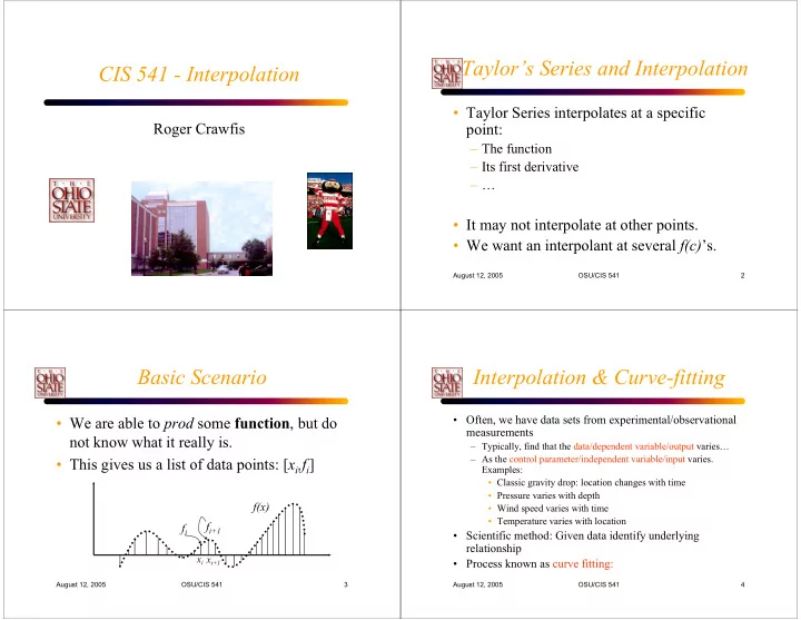
Taylor’s Series and Interpolation CIS 541 - Interpolation • Taylor Series interpolates at a specific Roger Crawfis point: – The function – Its first derivative – … • It may not interpolate at other points. • We want an interpolant at several f(c) ’s. August 12, 2005 OSU/CIS 541 2 Basic Scenario Interpolation & Curve-fitting • Often, we have data sets from experimental/observational • We are able to prod some function , but do measurements not know what it really is. – Typically, find that the data/dependent variable/output varies… – As the control parameter/independent variable/input varies. • This gives us a list of data points: [ x i ,f i ] Examples: • Classic gravity drop: location changes with time • Pressure varies with depth f(x) • Wind speed varies with time • Temperature varies with location f i+1 f i • Scientific method: Given data identify underlying relationship x i x i+1 • Process known as curve fitting: August 12, 2005 OSU/CIS 541 3 August 12, 2005 OSU/CIS 541 4
Interpolation & Curve-fitting Interpolation Vs Regression • Given a data set of n+1 points (x i ,y i ) identify a function • Distinctly different approaches depending on the quality of f(x) (the curve), that is in some (well-defined) sense the the data best fit to the data • Consider the pictures below: • Used for: extrapolate – Identification of underlying relationship (modelling/prediction) interpolate – Interpolation (filling in the gaps) extrapolate – Extrapolation (predicting outside the range of the data) Pretty confident: Unsure what the relationship is there is a polynomial relationship Clear scatter Little/no scatter Want to find an expression Want to find an expression that captures the trend: that passes exactly through all the points minimize some measure of the error Of all the points… August 12, 2005 OSU/CIS 541 5 August 12, 2005 OSU/CIS 541 6 Interpolation Interpolation • Concentrate first on the case where we believe there is no • Clearly, the crucial question is the selection of the error in the data (and round-off is assumed to be simple functions g(x) negligible). • Types are: • So we have y i =f(x i ) at n+1 points x 0 ,x 1 …x i ,…x n : x j > x j-1 • (Often but not always evenly spaced) – Polynomials • In general, we do not know the underlying function f(x) – Splines • Conceptually, interpolation consists of two stages: – Trigonometric functions – Develop a simple function g(x) that – Spectral functions…Rational functions etc… • Approximates f(x) • Passes through all the points x i – Evaluate f(x t ) where x 0 < x t < x n August 12, 2005 OSU/CIS 541 7 August 12, 2005 OSU/CIS 541 8
Curve Approximation Polynomial Interpolation • We will look at three possible • Consider our data set of n+1 points y i =f(x i ) at approximations (time permitting): n+1 points x 0 ,x 1 …x i ,…x n : x j > x j-1 – Polynomial interpolation • In general, given n+1 points, there is a – Spline (polynomial) interpolation unique polynomial g n (x) of order n: – Least-squares (polynomial) approximation = + + 2 + + n g ( ) x a a x a x a x K • If you know your function is periodic, then n 0 1 2 n trigonometric functions may work better. • That passes through all n+1 points – Fourier Transform and representations August 12, 2005 OSU/CIS 541 9 August 12, 2005 OSU/CIS 541 10 Polynomial Interpolation Polynomial Interpolation • There are a variety of ways of expressing • Existence – does there exist a polynomial the same polynomial that exactly passes through the n data points? • Lagrange interpolating polynomials • Uniqueness – Is there more than one such • Newton’s divided difference interpolating polynomial? polynomials – We will assume uniqueness for now and prove • We will look at both forms it latter. August 12, 2005 OSU/CIS 541 11 August 12, 2005 OSU/CIS 541 12
Lagrange Polynomials Linear Interpolation • Summation of terms, such that: • Summation of two lines: – Equal to f() at a data n ∑ 1 ∑ = p ( ) x L x f x ( ) ( ) = p x ( ) L x f x ( ) ( ) point. 1 i i n i i = i 0 = i 0 ( ) ( ) − − x x x x – Equal to zero at all ( ) = + 1 f x ( ) 0 f x ( ) − x x n ( ) ( ) ∏ − 0 − 1 x x x x other data points. = k L x ( ) 0 1 1 0 ( ) i − x x – Each term is a n th - = ≠ k 0, k i i k degree polynomial = ⎧ 1 i j Remember this when we = δ = ⎨ L x ( ) talk about piecewise-linear Existence!!! i j ij ≠ splines 0 i j ⎩ x 0 x 1 August 12, 2005 OSU/CIS 541 13 August 12, 2005 OSU/CIS 541 14 Lagrange Polynomials Lagrange Polynomials • 2 nd Order Case => quadratic polynomials • Sum must be a unique 2 nd order polynomial through all the data points. The first quadratic has roots The second quadratic has Adding them all together, The third quadratic has • What is an efficient implementation? at x 1 and x 2 and a value roots at x 0 and x 2 and a roots at x 0 and x 1 and a we get the interpolating value equal to the function equal to the function data value equal to the function quadratic polynomial, such data at x 2 . at x 0 . that: data at x 1 . • P(x 0 ) = 0 • P(x 0 ) = f 0 • P(x 0 ) = 0 • P(x 0 ) = f 0 • P(x 1 ) = 0 • P(x 1 ) = f 1 • P(x 1 ) = f 1 • P(x 1 ) = 0 • P(x 2 ) = f 2 • P(x 2 ) = 0 • P(x 2 ) = f 1 • P(x 2 ) = 0 x 0 x 2 x 1 August 12, 2005 OSU/CIS 541 15 August 12, 2005 OSU/CIS 541 16
Invariance Theorem Newton Interpolation • Consider our data set of n+1 points y i =f(x i ) at x 0 ,x 1 …x i ,…x n : x n > x 0 • Note, that the order of the data points does • Since p n (x) is the unique polynomial p n (x) of order n , write it: not matter. = + − + − − + + − − − p ( ) x b b x ( x ) b x ( x )( x x ) K b x ( x )( x x ) L ( x x ) − n 0 1 0 2 0 1 n 0 1 n 1 = b f x ( ) 0 0 • All that is required is that the data points are − f x ( ) f x ( ) [ ] = = b f x x , 1 0 1 1 0 − x x distinct. 1 0 − f x x [ , ] f x x [ , ] [ ] = = b f x x x , , 2 1 1 0 2 2 1 0 − x x • Hence, the divided difference f[x 0, x 1, … , x k ] 2 0 M is invariant under all permutations of the [ ] [ ] − f x , K , x f x , K , x [ ] = = n 1 n − 1 0 b f x , x , , x K n n n − 1 0 − x x x i ‘s. n 0 • f[x i ,x j ] is a first divided difference • f[x 2 ,x 1 ,x 0 ] is a second divided difference, etc. August 12, 2005 OSU/CIS 541 17 August 12, 2005 OSU/CIS 541 18 Linear Interpolation Quadratic Interpolation • Simple linear interpolation results from • Three data points: having only 2 data points. − f x ( ) f x ( ) = + − + − − p ( ) x f x ( ) 1 0 ( x x ) f x x x [ , , ]( x x )( x x ) − 2 0 − 0 0 1 2 0 1 x x f x ( ) f x ( ) 1 0 = + − p x ( ) f x ( ) 1 0 ( x x ) ⎡ ⎤ ⎡ ⎤ f x ( ) − f x ( ) f x ( ) − f x ( ) 1 0 − 0 x x − 2 1 1 0 ⎢ ⎥ ⎢ ⎥ f x ( ) − f x ( ) ⎣ − ⎦ ⎣ − ⎦ x x x x 1 0 = + − + − − f x ( ) ( x x ) ( x x )( x x ) 1 0 2 1 1 0 0 0 0 1 x − x − x x 1 0 2 0 slope − f x ( ) f x ( ) = + − f x ( ) 1 0 ( x x ) 0 0 − x x 1 0 ⎛ ⎡ ⎤ ⎞ ⎛ ⎡ ⎤ ⎞ − − f x ( ) f x ( ) ( f x ( ) f x ( ) − − − − − ⎜ 2 1 x x ) ( x x ) ⎟ ⎜ 1 0 ( x x ) ( x x ) ⎟ ⎢ ⎥ ⎢ ⎥ − 1 0 − 0 1 x x x x ⎝ ⎣ ⎦ ⎠ ⎝ ⎣ ⎦ ⎠ + 2 1 1 0 − x x x 0 x 1 2 0 August 12, 2005 OSU/CIS 541 19 August 12, 2005 OSU/CIS 541 20
Newton Interpolation Evaluating for x 2 ( ) ( )( ) = + − + − − f x ( ) b b x x b x x x x • Let’s look at the recursion formula: 2 0 1 2 0 2 2 0 2 1 ⎛ ⎞ [ ] [ ] − f f − f x , , x f x , , x K K ( ) ( ) [ ] = + − + − − = = n 1 n − 1 0 f b x x 2 1 b x x b f x , x , , x ⎜ ⎟ K − n n n 1 0 − x x 0 1 2 0 − 1 2 1 x x ⎝ ⎠ n 0 2 1 where = f x [ ] f x ( ) ( ) = + − + − f b x x f f i i 0 1 1 0 2 1 • For the quadratic term: ⎛ ⎞ − f f ( ) = + − + − − − f 1 0 x x f f f x ( ) f x ( ) f x ( ) f x ( ) ⎜ ⎟ − 2 1 1 0 0 − 1 0 2 1 x x ⎝ ⎠ − − − f x x [ , ] f x x [ , ] x x x x 1 0 [ ] = = 2 1 1 0 = 2 1 1 0 b f x x x , , = 2 2 1 0 − − f x x x x 2 0 2 0 2 − f x ( ) f x ( ) − 2 1 b 1 − x x = 2 1 − x x 2 0 August 12, 2005 OSU/CIS 541 21 August 12, 2005 OSU/CIS 541 22 Example: ln(x) Example: ln(x) • Interpolation of ln(2): given ln(1); ln(4) and ln(6) • Quadratic interpolation catches some – Data points: {(1,0), (4,1.3863), (6,1.79176)} of the curvature – Linear Interpolation: 0 + {(1.3863-0)/(4-1)}( x -1) = 0.4621( x -1) – Quadratic Interpolation: 0.4621( x -1)+((0.40546-1.3863)/2)( x -1)( x -4) • Improves the result somewhat = 0.4621( x -1) - 0.49( x -1)( x -4) • Not always a good idea: see later… Note the divergence for values outside of the data range. August 12, 2005 OSU/CIS 541 23 August 12, 2005 OSU/CIS 541 24
Recommend
More recommend
Explore More Topics
Stay informed with curated content and fresh updates.
