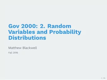
Lecture 2: Probability and Distributions Ani Manichaikul - PowerPoint PPT Presentation
Lecture 2: Probability and Distributions Ani Manichaikul amanicha@jhsph.edu 17 April 2007 1 / 65 Probability: Why do we care? Probability helps us by: Allowing us to translate scientific questions info mathematical notation Providing a
Lecture 2: Probability and Distributions Ani Manichaikul amanicha@jhsph.edu 17 April 2007 1 / 65
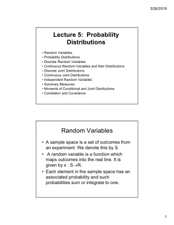
Probability: Why do we care? Probability helps us by: Allowing us to translate scientific questions info mathematical notation Providing a framework for answering scientific questions Later, we will see how some common statistical methods in the scientific literature are actually probability concepts in disguise 2 / 65
What is Probability? Probability is a measure of uncertainty about the occurrence of events Two definitions of probability Classical definition Relative frequency definition 3 / 65
Classical Definition P ( E ) = m N If an event can occur in N equally likely and mutually exclusive ways, and if m of these ways possess the characteristic E , then the probability of E is m N 4 / 65
Example: Coin toss Flip one coin Tails and heads equally likely N = 2 possible events Let H=Heads and T=Tails We are interested in the probability of tails: P (Tails)= P ( T ) = 1 2 5 / 65
Relative Frequency Definition P ( E ) = m n If an experiment is repeated n times, and characteristic E occurs m of those times, then the relative frequency of E is m n , and it is approximately equal to the probability of E 6 / 65
Example: Multiple coin tosses I Flip 100 coins Outcome Frequency T = Tails 53 H = Heads 47 Total 100 P (Tails) = P ( T ) ≈ 53 100 = 0 . 53 ≈ 0 . 50 7 / 65
Example: Multiple coin tosses II What happens if we flip 10,000 coins? Outcome Frequency T = Tails 5063 H = Heads 4937 Total 10000 P (Tails) = P ( T ) ≈ 5063 10000 = 0 . 51 ≈ 0 . 50 8 / 65
Relative frequency intuition The probability of T is the limit of the relative frequency of T, as the sample size n goes to infinity “The long run relative frequency” 9 / 65
Outcome characteristics Statistical independence Mutually exclusive 10 / 65
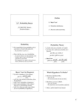
Statistical Independence Two events are statistically independent if the joint probability of both events occurring is the product of the probabilities of each event occuring: P ( A and B ) = P ( A ) × P ( B ) 11 / 65
Example Let A = first born child is female Let B = second child is female P(A and B) = probability that first and second children are both female: Assuming independence: P ( A and B ) = P ( A ) × P ( B ) = 1 2 × 1 2 = 1 4 12 / 65
Statistical independence: comment “In a study where we are selecting patients at random from a population of interest, we assume that the outcomes we observe are independent...” In what situations would this assumption be violated 13 / 65
Mutually exclusive Two events are mutually exclusive if the joint probability of both events occuring is 0: P ( A and B ) = 0 Ex: A = first child is female, B = first child is male 14 / 65
Probability rules 1 The probability of any event is non-negative, and no greater than 1: 0 ≤ P ( E ) ≤ 1 2 Given n mutually exclusive events, E 1 , E 2 , · · · , E n covering the sample space, the sum of the probabilities of events is 1: n � P ( E i ) = P ( E 1 ) + P ( E 2 ) + · · · + P ( E n ) = 1 i =1 3 If E i and E j are mutually exclusive events, then the probability that either E i or E j occur is: P ( E i ∪ E j ) = P ( E i ) + P ( E j ) 15 / 65
Set notation A set is a group of disjoint objects An element of a set is an object in the set The union if two sets, A and B, is a larger set that contains all elements in either A, B or both Notation: A ∪ B The intersection if two sets, A and B, is the set containing all elements found in both A and B Notation: A ∩ B 16 / 65
The addition rule If two events, A and B, are not mutually exclusive, then the probability that event A or event B occurs is: P ( A ∪ B ) = P ( A ) + P ( B ) − P ( A ∩ B ) where P ( A ∩ B ) is the probability that both events occur 17 / 65
Conditional probability The conditional probability of an event A given an event B is: P ( A | B ) = P ( A ∩ B ) P ( B ) where P ( B ) � = 0 18 / 65
The multiplication rule In general: P ( A ∩ B ) = P ( B ) × P ( A | B ) When events A and B are independent, P ( A | B ) = P ( A ) and: P ( A ∩ B ) = P ( A ) × P ( B ) 19 / 65
Bayes rule Useful for computing P ( B | A ) if P ( A | B ) and P ( A | B c ) are known Ex: Screening We know P (test positive | true positive) We want P (true positive | test positive) Ex: Bayesian statistics uses assumptions about P (data | state of the world) to derive statements about P (state of the world | data) The rule: P ( A | B ) · P ( B ) P ( B | A ) = P ( A | B ) · P ( B ) + P ( A | B c ) · P ( B c ) where B c denotes “the complement of B” or “not B” 20 / 65
Example: Sex and Age I Age Age Young ( B 1 ) Older ( B 2 ) Total Male ( A 1 ) 30 20 50 Female ( A 2 ) 40 10 50 Total 70 30 100 21 / 65
Example: Sex and Age II A 1 = { all males } , A 2 = { all females } B 1 = { all young } , B 2 = { all older } A 1 ∪ A 2 = { all people } = B 1 ∪ B 2 A 1 ∩ A 2 = { no people } = ∅ = B 1 ∩ B 2 A 1 ∪ B 1 = { all males and young females } A 1 ∪ B 2 = { all males and older females } A 2 ∩ B 2 = { older females } 22 / 65
Example: Sex and Age III P (male) = 50 P ( A 1 ) = 100 = 0 . 5 P (female) = 50 P ( A 2 ) = 100 = 0 . 5 P (young) = 70 P ( B 1 ) = 100 = 0 . 7 P (older) = 30 P ( B 2 ) = 100 = 0 . 3 23 / 65
Example: Sex and Age IV P (older and female) = 10 P ( A 2 ∩ B 2 ) = 100 = 0 . 1 P ( A 1 ∪ B 1 ) = P (young or male) P ( A 1 ) + P ( B 1 ) − P ( A 1 ∩ B 1 ) = 100 + 70 50 100 − 30 = 100 90 = 100 = 0 . 9 24 / 65
Example: Sex and Age V P ( B 2 | A 2 ) P (older | female) = P ( B 2 ∩ A 2 ) = 10 / 100 50 / 100 = 10 = 50 = 0 . 2 P ( A 2 ) P ( B 2 | A 1 ) P (older | male) = P ( B 2 ∩ A 1 ) = 20 / 100 50 / 100 = 20 = 50 = 0 . 4 P ( A 1 ) P (older) = 30 P ( B 2 ) = 100 = 0 . 3 P ( B 2 | A 2 ) � = P ( B 2 | A 1 ) � = P ( B 2 ) → In this group, sex and age are not independent 25 / 65
Example: Sex and Age VI P ( A 1 ∪ A 2 ) = P ( B 1 ∪ B 2 ) = P ( A 2 | B 2 ) = 26 / 65
Example: Blood Groups I Sex Blood group Male Female Total O 113 170 283 A 103 155 258 B 25 37 62 AB 10 15 25 Total 251 377 628 27 / 65
Example: Blood Groups II 1 − P (female) = 251 628 ≈ 0 . 4 P (male) = 283 628 ≈ 0 . 45 P ( O ) = 258 P ( A ) = 628 ≈ 0 . 41 62 628 ≈ 0 . 10 P ( B ) = 25 628 ≈ 0 . 04 P ( AB ) = 28 / 65
Example: Blood Groups III Question: Are sex and blood group independent? 113 P ( O | male) = 251 ≈ 0 . 45 170 P ( O | female) 377 ≈ 0 . 45 = 283 628 ≈ 0 . 45 same as P ( O ) = Can show same equalities for all blood types → Yes, sex and blood group appear to be independent of each other in this sample 29 / 65
Example: Disease in the population I For patients with Disease X, suppose we knew the age proportions per sex, as well as the sex distribution. Question: Could we compute the sex proportions in each age group (young / older)? Answer: Use Bayes Rule 30 / 65
Example: Disease in the population II P ( A 1 ) = P ( A 2 ) = 0 . 5 P ( B 2 | A 2 ) = 0 . 2 P ( B 2 | A 1 ) = 0 . 4 P ( B 2 | A 2 ) · P ( A 2 ) P ( A 2 | B 2 ) = P ( B 2 | A 2 ) · P ( A 2 ) + P ( B 2 | A 1 ) · P ( A 1 ) 31 / 65
Probability Distributions Often, we assume a true underlying distribution Ex: P (tails) = 1 2 , P (heads) = 1 2 This distribution is characterized by a mathermatical formula and a set of possible outcomes Two types of distributions: Discrete Continuous 32 / 65
Most Commonly Used Discrete Distributions Binomial – two possible outcomes Underlies much of statistical applications to epidemiology Basic model for logistic regression Poisson – uses counts of events of rates Basis for log-linear models 33 / 65
Most Commonly Used Continuous Distributions Normal – bell shaped curve Many characteristics are normally distributed or approximately normally distributed Basic model for linear regression Exponential – useful in describing growth 34 / 65
Counting techniques Factorials: counts the number of ways to arrange things Permutations: counts the number of possible ordered arrangements of subsets Combinations: counts the number of possible unordered arrangements of subsets 35 / 65
Factorials Notation: n! (“n factorial”) Number of possible arrangements of n objects n! = n(n-1)(n-2)(n-3) · · · (3)(2)(1) 36 / 65
Permutations Ordered arrangement of n objects, taken r at a time n ! = n P r ( n − r )! n ( n − 1) · · · ( n − r + 1)( n − r ) · · · 1 = ( n − r )( n − r − 1) · · · 1 n ( n − 1)( n − 2) · · · ( n − r + 1) = 37 / 65
Combinations An arragement of n objects taken r at a time without regard to order � n � n ! = “n choose r” = r !( n − r )! r � 4 � 2!(4 − 2)! = 4 · 3 · 2 · 1 4! = 12 = 2 = 6 2! · 2! 2 Note: the number of combinations is less than or equal to the number of permutations. 38 / 65
The Binomial Distribution You’ve seen it before: 2 x 2 tables and applications Proportions: CIs and tests Sensitivity and Specificity Odds ratio and relative risk Logistic regression 39 / 65
Recommend
More recommend
Explore More Topics
Stay informed with curated content and fresh updates.
