Lecture 2: January 29 and Feb 3 Information Textbook issues resolved? - PDF document

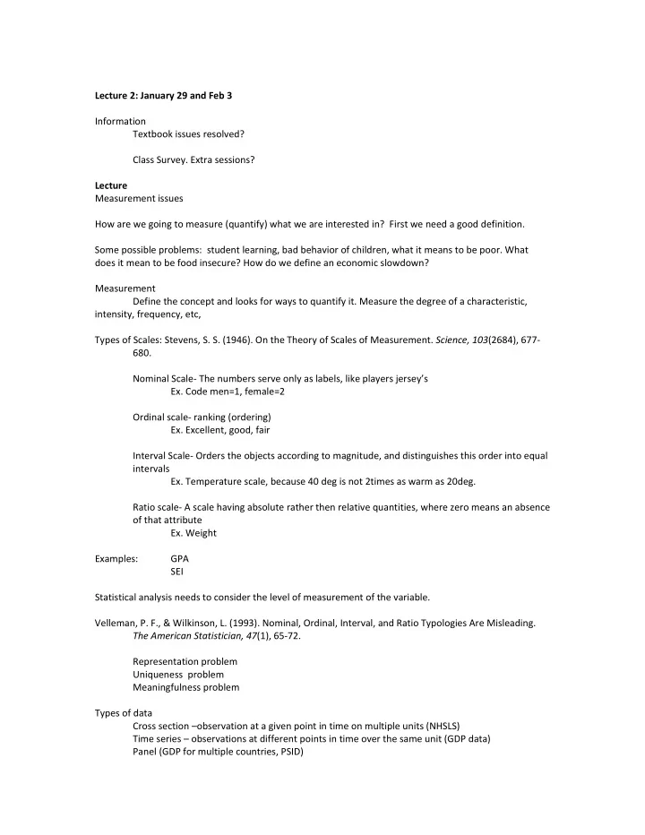
Lecture 2: January 29 and Feb 3 Information Textbook issues resolved? Class Survey. Extra sessions? Lecture Measurement issues How are we going to measure (quantify) what we are interested in? First we need a good definition. Some possible problems: student learning, bad behavior of children, what it means to be poor. What does it mean to be food insecure? How do we define an economic slowdown? Measurement Define the concept and looks for ways to quantify it. Measure the degree of a characteristic, intensity, frequency, etc, Types of Scales: Stevens, S. S. (1946). On the Theory of Scales of Measurement. Science, 103 (2684), 677 ‐ 680. Nominal Scale ‐ The numbers serve only as labels, like players jersey’s Ex. Code men=1, female=2 Ordinal scale ‐ ranking (ordering) Ex. Excellent, good, fair Interval Scale ‐ Orders the objects according to magnitude, and distinguishes this order into equal intervals Ex. Temperature scale, because 40 deg is not 2times as warm as 20deg. Ratio scale ‐ A scale having absolute rather then relative quantities, where zero means an absence of that attribute Ex. Weight Examples: GPA SEI Statistical analysis needs to consider the level of measurement of the variable. Velleman, P. F., & Wilkinson, L. (1993). Nominal, Ordinal, Interval, and Ratio Typologies Are Misleading. The American Statistician, 47 (1), 65 ‐ 72. Representation problem Uniqueness problem Meaningfulness problem Types of data Cross section –observation at a given point in time on multiple units (NHSLS) Time series – observations at different points in time over the same unit (GDP data) Panel (GDP for multiple countries, PSID)

Longitudinal (NLSY) Repeated cross section (same data, but different cross sectional units at each time period. Ex CPS, GSS) I’ll start with some basic terminology that’s relevant to longitudinal data. First, the term ‘longitudinal data’ is somewhat vague. Generally, the term implies that one has panel data, that is, data collected on multiple units across multiple points in time (like the PSID). However, it is often also used to refer to repeated cross ‐ sectional data, that is, data collected on multiple different units at multiple points in time (like the GSS). A basic model: Exam Score = f(X??) hours spent studying, IQ, ACT, Gender?, Age? Major? GDP Growth = f (x??) Investment growth, Democracy, Political Stability, Corruption, Endogenous (explained) = Function of Exogenous (explanatory) Left Hand Side (LHS) = Right hand side (RHS) Some other ways of classifying data: For the most part RHS data can be of any type, but different left hand side variables often dictate different models. Some common types of data and their models. Interval and ratio data as LHS variable are often candidates for Linear Regression Dichotomous Choice, Binomial, discrete. Taking on just two values, 1 or 0, yes or no are often estimated using logit or probit models. These are often nominal variables, which take only two values. Multinomial Logit models are often used for dependent variables that are nominal but include more than two choices. For example if you were trying to estimate (explain) a person’s choice of transportation, where the choices could be bike, car, bus, subway. Ordinal dependent variables are often estimated with Ordered Probit or Ordered Logit Count Data. The number of events, for example the number of car accident someone has had or the number of drinks. Ie the data are not continuous. Typically there are respondents with 0 events. One method of estimating theses models is the Poisson Regression, since a Poisson distribution better represents the data. But there are some crucial aspects to this such as the degree of dispersion and the number of zeros. There are other methods of Poisson isn’t the best fitting like negative binomial or a Hurdle model. Interval Regression. A better way of handling variables that are in fact intervals. For example: Lets say you ask “What is your annual gross income?” and offer the following categories: 1. $0 ‐ 10,000 2. $10,001 ‐ $50,000 3. $50,001 ‐ 100,000 4. $100,001 + Duration Data the time it takes for something to happen, such as an event. Related to the probit and logit models in those models you predict if the event happens or does not. Data Censoring and Truncation. Censoring – recording a value that is not the true value, through setting an upper or lower limit. The income variable above is right censored if we recorded 100,000 for everyone who said 100,000 + Truncating is when data is not recorded at all, say due to inability to measure it at certain levels.

For your projects you want to find an interval or ration scaled variable to explain, in other words to be the LHS variable. Data Sources: This link provides a good list http://www.oswego.edu/~economic/data.htm

Review Basic Stats I will be using data from DeMaris (2004) on faculty salaries. Descriptive vs inferential stats Descriptive Statistics Statistics is broken into two branches Descriptive Statistics ‐ describe the data collected Inferential Statistics – draw inferences about the population from which the sample was drawn Some quick notes: Deciding on the appropriate statistical test requires understanding the level of measurement and the type of variable. categorical(discreet) vs. continuous nominal, ordinal, interval and ratio Conventions: I will try and use Latin letters to represent sample statistics, I will also use Greek letters to represent population parameters. Estimates of population parameters are often represented with a ^ (pronounced hat) over the letter. Descriptive Statistics Describing the data you’ve collected Univariate single variable Frequency distributions (categorical) count Relative frequency (percentage) distributions valid percent total percent Proportion Other ways of describing the distribution 3 Measures of Central tendency 1. Mean ‐ sometime called the first moment n   x      i x x ... x   i 1 1 2 n x n n 2. Median – When the data is ordered largest to smallest it is the middles number if there are an odd number, and the mean of the middle two if there are an even number. The 50 th percentile 3. Mode – the most frequently occurring 4. Trimmed mean (delete upper and lower % and calculate mean)

When are the mean and median different why might you prefer one to the other. When might you use the mode? SPSS Demo Measures of Dispersion (spread) Range – highest – lowest value Variance ‐ sometimes called the second moment n    2 ( x x ) i  2 i 1 s  n 1 Standard Deviation n   2 ( x x ) i    2 i 1 s s  n 1  1 1 Tchebysheff’s theorem: for k>1 for any distribution. Where k represents the number of 2 k standard deviations. So 3/4 of the values lie within 2 standard deviations Empirical rule: 68% lie +/ ‐ 1 s.d., 95% lie +/ ‐ 2 s.d. Measures of Shape Skewness (third moment) Positive Skew long tail to right      3 X  3 N Kurtosis (fourth moment) measure of the size of tails Leptokurtic, fat tails >0 Platykurtic small tails <0      4 X  3  4 N Graphical Representation of Univariate descriptive stats Categorical Bar Chart Pie Chart Continuous Histogram Line Chart Bok and Whiskers The following example uses SPSS syntax to generate some descriptive statistics from above. This is done using the DeMaris (2004) dataset for faculty salaries. salary: Academic year (9 month) salary in US dollars market: the ratio of average national salary for the discipline to average salary of all disciplines. male: dummy variable (indicator variable) 1=male 0=female yearsdg: time since degree in years

GET FILE='C:\Documents and Settings\brooks.tagg\My Documents\Classes\ECO 307\data\faculty.sav'. DATASET NAME DataSet2 WINDOW=FRONT. DESCRIPTIVES VARIABLES=salary /STATISTICS=MEAN STDDEV MIN MAX SKEWNESS KURTOSIS. Descriptive Statistics N Minimum Maximum Mean Std. Deviation salary 514 29000.00 96156.00 50863.8734 12672.77130 514 Valid N (listwise) Descriptive Statistics N Skewness Kurtosis Statistic Statistic Std. Error Statistic Std. Error salary 514 .449 .108 -.235 .215 Valid N (listwise) 514 EXAMINE VARIABLES=salary BY male /PLOT=BOXPLOT /STATISTICS=NONE /NOTOTAL.

GRAPH /TITLE='Histogram of Academic Salary' /FOOTNOTE='Footnote Data are from DeMaris (2004)' /HISTOGRAM=salary /PANEL ROWVAR=male ROWOP=CROSS.

Lecture 3: Univariate and Bivariate Bivariate Descriptive statistics 2 variables 3 possible combinations Categorical/Categorical Crosstabulations (2 way frequency tables, Crosstabs, Bivariate distributions) Example: Smoke\Gender Male Female Row total Yes 30 25 55 No 20 25 45 column total 50 50 100 Categorical/Continuous Any statistic that applied to cont. variables done for each category Continuous/Continuous Simple Correlation coefficient (Pearson’s product ‐ moment correlation coefficient, Covariance)    ( x x )( y y )   i i r r   xy yx   2 2 ( x x ) ( y y ) i i this ranges from +1 to ‐ 1 Graphical Representations Bar Charts pie charts etc. histogram, box plots scatter plots Inferential Statistics http://www.ruf.rice.edu/~lane/stat_sim/sampling_dist/index.html To draw inference from a sample about the properties of a population Population distribution: The distribution of a given variable(parameter) for the entire population Sample distribution: A sample of size n, is drawn from the population and the variable’s distribution is called the sample distribution.