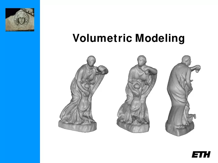

Volumetric Modeling
Schedule (tentative) Feb 18 Introduction Feb 25 Lecture: Geometry, Camera Model, Calibration Mar 4 Lecture: Features, Tracking/Matching Project Proposals by Students Mar 11 Mar 18 Lecture: Epipolar Geometry Mar 25 Lecture: Stereo Vision Apr 1 Easter Apr 8 Short lecture “Stereo Vision (2)” + 2 papers Project Updates Apr 15 Apr 22 Short lecture “Active Ranging, Structured Light” + 2 papers Short lecture “Volumetric Modeling” + 1 paper Apr 29 May 6 Short lecture “Mesh-based Modeling” + 2 papers May 13 Lecture: Structure from Motion, SLAM May 20 Pentecost / White Monday May 27 Final Demos
Today’s class Modeling 3D surfaces by means of a discretized volume grid. In particular: • extracting a triangular mesh from an implicit volume representation • volumetric range image integration • convex 3D shape modeling
Volumetric Representation • Sample a volume containing the surface of interest uniformly • Label each grid point as lying inside or outside the surface, e.g. by defining a signed distance function (SDF) with positive values inside and negative values outside • The modeled surface is represented as an isosurface of the labeling (implicit) function
Volumetric Representation • Why volumetric modeling? • G ives a flexible and robust surface representation • Handles complex surface topologies effortlessly • Allows to sample the entire volume of interest by storing information about space opacity • Offers possibilities for parallel computing
From volume to mesh: Marching Cubes “Marching Cubes: A High Resolution 3D Surface Construction Algorithm”, William E. Lorensen and Harvey E. Cline, Computer Graphics (Proceedings of SIGGRAPH '87). • Basic idea: March through the volume and process each voxel by determining all potential intersection points of its edges with the desired isosurface; precise localization via interpolation • Obtained intersection points serve as vertices of triangles which make up a triangulation of the constructed isosurface
From volume to mesh: Marching Cubes Example: “Marching Squares” in 2D
From volume to mesh: Marching Cubes By summarizing symmetric configurations, all possible 2 8 = 256 cases reduce to:
From volume to mesh: Marching Cubes • The accuracy of the computed surface depends on the volume resolution • Precise normal specification at each vertex possible by means of the implicit function
From volume to mesh: Marching Cubes • Benefits of Marching Cubes • Always generates a manifold surface • The desired sampling density can easily be controlled • Trivial merging or overlapping of different surfaces based on the corresponding implicit functions: minimum of the values for merging and averaging for overlapping
From volume to mesh: Marching Cubes • Limitations of Marching Cubes • Maintains a 3D entry rather than 2D which entails considerable computational and memory requirements • Generates consistent topology, but not always the topology you wanted • Problems with very thin surfaces
Range Image Integration “A Volumetric Method for Building Complex Models from Range Images”, Brian Curless and Marc Levoy, Computer Graphics (Proceedings of SIGGRAPH ‘96). • Generate a signed distance function (or something close to it) for each scan • Compute a weighted average • Extract isosurface
Range Image Integration range surfaces signed distance volume to surface weight (~accuracy) distance depth sensor surface1 • use voxel space • new surface as zero-crossing (find using marching cubes) surface2 • least-squares estimate combined estimate (zero derivative=minimum)
Range Image Integration It turns out that the least-squares estimate leads to the following simple fusion scheme: 𝑋 𝑗 𝑦 𝐸 𝑗 𝑦 + 𝑥 𝑗+1 ( 𝑦 ) 𝑒 𝑗+1 ( 𝑦 ) 𝐸 𝑗+1 𝑦 = 𝑋 𝑗 𝑦 + 𝑥 𝑗+1 ( 𝑦 ) 𝑋 𝑗+1 𝑦 = 𝑋 𝑗 𝑦 + 𝑥 𝑗+1 𝑦 , where 𝑒 𝑗 and 𝑥 𝑗 denote the depth map and weighting function to range image 𝑗 , and 𝐸 𝑗 and 𝑋 𝑗 denote the accumulated measures.
Range Image Integration Depth maps and weighting functions are computed with a ray casting procedure and linear interpolation within intersected triangles
KinectFusion “KinectFusion: Real-Time Dense Surface Mapping and Tracking”, R. Newcombe, S. Izadi, O. Hilliges, D. Molyneaux, D. Kim, A. Davison, P . Kohli, J. Shotton, S. Hodges, A. Fitzgibbon IEEE International Symposium on Mixed and Augmented Reality, ISMAR, 2011. • Camera pose estimation via multi-resolution ICP • Surface prediction by ray casting the current 3D reconstruction • Volumetric integration of all depth measurements via a single TSDF • Uses GPU to accelerate volumetric integration step and reach real-time performance
KinectFusion ⇒ video: http://research.microsoft.com/apps/video/default.aspx?id= 152815
Kintinuous “Kintinuous: Spatially Extended KinectFusion”, T. Whelan, M. Kaess, M. F . Fallon, H. Johannsson, J. J. Leonard, J. M. McDonald RSS Workshop on RGB-D: Advanced Reasoning with Depth Cameras, 2012. • Capable of reconstructing large-scale environments by shifting the volume of interest in space
Convex 3D Modeling “Continuous Global Optimization in Multiview 3D Reconstruction”, Kalin Kolev, Maria Klodt, Thomas Brox and Daniel Cremers, International Journal of Computer Vision (IJCV ‘09). • Multiview stereo allows to compute entities of the type: • ρ ∶ 𝑊 → [0,1] photoconsistency map reflecting the agreement of corresponding image projections 𝑔 ∶ 𝑊 → [0,1] potential function representing the costs for • a voxel for lying inside the surface • How can these measures be integrated in a consistent and robust manner?
Convex 3D Modeling • Photoconsistency is usually computed by matching corresponding image projections in different views • Instead of comparing only the pixel colors, image patches are considered around each point to reach better robustness • Challenges: • Many real-world objects do not satisfy the underlying Lambertian assumption • Matching is ill-posed, as there are usually a lot of different potential matches among multiple views • Visibility
Convex 3D Modeling A potential function 𝑔 ∶ 𝑊 → • [0,1] can be obtained by fusing multiple depth maps or with a direct 3D approach • Depth map estimation is fast but leads to a two-step method (disadvantage: errors could propagate and degrade the final result) • The direct approach is generally computationally more intense but offers more robustness and flexibility (occlusion handling, projective patch distortion etc.) • Proposed propagation scheme entails additional advantages by the possibility to define a sharp deblurred photoconsistency map via a voting strategy
Convex 3D Modeling Example: Middlebury “dino” data set ρ f
Convex 3D Modeling By introducing a binary labeling function 𝑣 ∶ 𝑊 → {0,1} reflecting the indicator function of the interior region, the modeling problem can be cast as minimizing 𝐹 𝑣 = � ρ 𝛼𝑣 𝑒𝑦 + λ � 𝑔 𝑣 𝑒𝑦 𝑊 𝑊 over the set 𝐷 𝑐𝑗𝑐 = 𝑣 𝑣 ∶ 𝑊 → 0,1 } . One can observe that the above functional is convex, but it is optimized over a non-convex domain. A constrained convex optimization problem can be derived by relaxing the binary condition to 𝐷 𝑠𝑠𝑠 = 𝑣 𝑣 ∶ 𝑊 → [0,1] } . Theorem: A global minimum of 𝐹 over 𝐷 𝑐𝑗𝑐 can be obtained by minimizing over 𝐷 𝑠𝑠𝑠 and thresholding the solution at some 𝑢𝑢𝑢 ∈ (0,1) .
Convex 3D Modeling • Properties of Total Variation (TV) 𝑈𝑊 𝑣 = � 𝛼𝑣 𝑒𝑦 𝑊 • preserves edges and discontinuities 𝑈𝑊 𝑔 1 = 𝑈𝑊 𝑔 2 = 𝑈𝑊 𝑔 3 • coarea formula ∞ 𝑈𝑊 𝑣 = � 𝑚𝑚𝑚𝑚𝑢𝑢 ( 𝑣 = λ ) 𝑒λ −∞
Convex 3D Modeling input images (2/28) input images (2/38)
Convex 3D Modeling • Benefits of the model • High-quality 3D reconstructions of sufficiently textured objects possible • Allows global optimizability • Simple construction without multiple processing stages and heuristic parameters • Computational time depends only on the volume resolution and not on the resolution of the input images • Perfectly parallelizable
Convex 3D Modeling • Limitations of the model • Computationally intense: computational time could exceed two hours on a single-core CPU depending on the utilized volume resolution • It may not be possible to compute an accurate potential function 𝑔 for objects strongly violating the Lambertian assumption
Convex 3D Modeling “Integration of Multiview Stereo and Silhouettes via Convex Functionals on Convex Domains”, Kalin Kolev and Daniel Cremers, European Conference on Computer Vision (ECCV ‘08). • Idea: Extract the silhouettes of the imaged object and use them as constraints to restrict the domain of feasible shapes
Recommend
More recommend