Lecture 17: Boosting CS109A Introduction to Data Science Pavlos - PowerPoint PPT Presentation
Lecture 17: Boosting CS109A Introduction to Data Science Pavlos Protopapas and Kevin Rader CS109B, STAT121B, AC209B CS109A, P ROTOPAPAS , R ADER 2 Outline Review of Ensemble Methods Finish Random Forest Boosting Gradient
Lecture 17: Boosting CS109A Introduction to Data Science Pavlos Protopapas and Kevin Rader
CS109B, STAT121B, AC209B CS109A, P ROTOPAPAS , R ADER 2
Outline • Review of Ensemble Methods • Finish Random Forest • Boosting • Gradient Boosting • Set-up and intuition • Connection to Gradient Descent • The Algorithm AdaBoost • CS109A, P ROTOPAPAS , R ADER 3
Bags and Forests of Trees • Last time we examined how the short-comings of single decision tree models can be overcome by ensemble methods - making one model out of many trees. • We focused on the problem of training large trees, these models have low bias but high variance. • We compensated by training an ensemble of full decision trees and then averaging their predictions - thereby reducing the variance of our final model. CS109A, P ROTOPAPAS , R ADER 4
Bags and Forests of Trees (cont.) Bagging: • create an ensemble of trees, each trained on a bootstrap sample of the training set • average the predictions. Random forest: • create an ensemble of trees, each trained on a bootstrap sample of the training set • in each tree and each split, randomly select a subset of predictors, choose a predictor from this subset for splitting • average the predictions Note that the ensemble building aspects of both methods are embarrassingly parallel! CS109A, P ROTOPAPAS , R ADER 5
Tuning Random Forests Random forest models have multiple hyper-parameters to tune: 1. the number of predictors to randomly select at each split 2. the total number of trees in the ensemble 3. the minimum leaf node size In theory, each tree in the random forest is full, but in practice this can be computationally expensive (and added redundancies in the model), thus, imposing a minimum node size is not unusual. CS109A, P ROTOPAPAS , R ADER 6
Tuning Random Forests There are standard (default) values for each of random forest hyper- parameters recommended by long time practitioners, but generally these parameters should be tuned through OOB (making them data and problem dependent). e.g. number of predictors to randomly select at each split: √𝑂 – # for classification $ – % for regression Using out-of-bag errors, training and cross validation can be done in a single sequence - we cease training once the out-of-bag error stabilizes CS109A, P ROTOPAPAS , R ADER 7
Variable Importance for RF Same as with Bagging: Calculate the total amount that the RSS (for regression) or Gini index (for classification) is decreased due to splits over a given predictor, averaged over all 𝐶 trees. CS109A, P ROTOPAPAS , R ADER 8
Variable Importance for RF Alternative: • Record the prediction accuracy on the oob samples for each tree. • Randomly permute the data for column 𝑘 in the oob samples the record the accuracy again. • The decrease in accuracy as a result of this permuting is averaged over all trees, and is used as a measure of the importance of variable 𝑘 in the random forest. CS109A, P ROTOPAPAS , R ADER 9
Variable Importance for RF 100 trees, max_depth=10 CS109A, P ROTOPAPAS , R ADER 10
Variable Importance for RF 100 trees, max_depth=10 CS109A, P ROTOPAPAS , R ADER 11
Final Thoughts on Random Forests When the number of predictors is large, but the number of relevant predictors is small, random forests can perform poorly. Question : Why? In each split, the chances of selected a relevant predictor will be low and hence most trees in the ensemble will be weak models. CS109A, P ROTOPAPAS , R ADER 12
Final Thoughts on Random Forests (cont.) Increasing the number of trees in the ensemble generally does not increase the risk of overfitting. Again, by decomposing the generalization error in terms of bias and variance, we see that increasing the number of trees produces a model that is at least as robust as a single tree. However, if the number of trees is too large, then the trees in the ensemble may become more correlated, increase the variance. CS109A, P ROTOPAPAS , R ADER 13
Final Thoughts on Random Forests (cont.) Probabilities: • Random Forrest Classifier (and bagging) can return probabilities. • Question : How? More questions Unbalance dataset? • GO TO THE ADVANCED TOPICS LATER TODAY • Weighted samples? • Categorical data? Missing data? • • Different implementations? CS109A, P ROTOPAPAS , R ADER 14
Boosting CS109A, P ROTOPAPAS , R ADER 15
Motivation for Boosting Question: Could we address the shortcomings of single decision trees models in some other way? For example, rather than performing variance reduction on complex trees, can we decrease the bias of simple trees - make them more expressive? A solution to this problem, making an expressive model from simple trees, is another class of ensemble methods called boosting . CS109A, P ROTOPAPAS , R ADER 16
Boosting Algorithms CS109A, P ROTOPAPAS , R ADER 17
Gradient Boosting The key intuition behind boosting is that one can take an ensemble of simple models { T h } h ∈ H and additively combine them into a single, more complex model. Each model T h might be a poor fit for the data, but a linear combination of the ensemble can be expressive/flexible. Question: But which models should we include in our ensemble? What should the coefficients or weights in the linear combination be? CS109A, P ROTOPAPAS , R ADER 18
Gradient Boosting: the algorithm Gradient boosting is a method for iteratively building a complex regression model T by adding simple models. Each new simple model added to the ensemble compensates for the weaknesses of the current ensemble. 1. Fit a simple model 𝑈 (,) on the training data { 𝑦 0 , 𝑧 0 , … , (𝑦 $ , 𝑧 $ )} Set 𝑈 ← 𝑈 (,) . Compute the residuals { r 1 , . . . , r N } for T . 2. Fit a simple model, 𝑈 (0) , to the current residuals , i.e. train using { 𝑦 0 , 𝑠 0 , … , (𝑦 $ , 𝑠 $ )} 3. Set 𝑈 ← 𝑈 + 𝜇𝑈 (0) 9 − 𝜇𝑈 ; 𝑦 9 , 𝑜 = 1, … , 𝑂 4. Compute residuals, set 𝑠 9 ← 𝑠 5. Repeat steps 2-4 until stopping condition met. where 𝜇 is a constant called the learning rate . CS109A, P ROTOPAPAS , R ADER 19
Gradient Boosting: illustration CS109A, P ROTOPAPAS , R ADER 20
Gradient Boosting: illustration CS109A, P ROTOPAPAS , R ADER 21
Gradient Boosting: illustration CS109A, P ROTOPAPAS , R ADER 22
Gradient Boosting: illustration CS109A, P ROTOPAPAS , R ADER 23
Gradient Boosting: illustration CS109A, P ROTOPAPAS , R ADER 24
Gradient Boosting: illustration CS109A, P ROTOPAPAS , R ADER 25
Why Does Gradient Boosting Work? Intuitively, each simple model T ( i ) we add to our ensemble model T , models the errors of T . Thus, with each addition of T ( i ) , the residual is reduced 9 − 𝜇𝑈 ; (𝑦 9 ) 𝑠 Note that gradient boosting has a tuning parameter, 𝜇 . If we want to easily reason about how to choose 𝜇 and investigate the effect of 𝜇 on the model T , we need a bit more mathematical formalism. In particular, how can we effectively descend through this optimization via an iterative algorithm? We need to formulate gradient boosting as a type of gradient descent . CS109A, P ROTOPAPAS , R ADER 26
Review: A Brief Sketch of Gradient Descent In optimization, when we wish to minimize a function, called the objective function , over a set of variables, we compute the partial derivatives of this function with respect to the variables . If the partial derivatives are sufficiently simple, one can analytically find a common root - i.e. a point at which all the partial derivatives vanish; this is called a stationary point . If the objective function has the property of being convex , then the stationary point is precisely the min. CS109A, P ROTOPAPAS , R ADER 27
Review: A Brief Sketch of Gradient Descent the Algorithm In practice, our objective functions are complicated and analytically find the stationary point is intractable. Instead, we use an iterative method called gradient descent : 1. Initialize the variables at any value: 2. Take the gradient of the objective function at the current variable values: 3. Adjust the variables values by some negative multiple of the gradient: The factor 𝜇 is often called the learning rate. CS109A, P ROTOPAPAS , R ADER 28
Why Does Gradient Descent Work? Claim: If the function is convex, this iterative methods will eventually move x close enough to the minimum, for an appropriate choice of 𝜇 . Why does this work? Recall, that as a vector, the gradient at at point gives the direction for the greatest possible rate of increase. CS109A, P ROTOPAPAS , R ADER 29
Why Does Gradient Descent Work? Subtracting a 𝜇 multiple of the gradient from x, moves x in the opposite direction of the gradient (hence towards the steepest decline) by a step of size 𝜇 . If f is convex, and we keep taking steps descending on the graph of f , we will eventually reach the minimum. CS109A, P ROTOPAPAS , R ADER 30
Gradient Boosting as Gradient Descent Often in regression, our objective is to minimize the MSE Treating this as an optimization problem, we can try to directly minimize the MSE with respect to the predictions The update step for gradient descent would look like CS109A, P ROTOPAPAS , R ADER 31
Recommend
More recommend
Explore More Topics
Stay informed with curated content and fresh updates.

