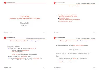
STK-IN4300 Statistical Learning Methods in Data Science - PowerPoint PPT Presentation
STK-IN4300 - Statistical Learning Methods in Data Science Outline of the lecture Gradient Boosting review L 2 boosting with linear learner STK-IN4300 Statistical Learning Methods in Data Science Likelihood-based Boosting introduction
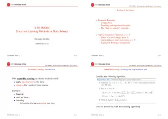
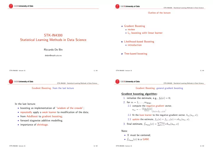
STK-IN4300 - Statistical Learning Methods in Data Science Outline of the lecture Gradient Boosting review L 2 boosting with linear learner STK-IN4300 Statistical Learning Methods in Data Science Likelihood-based Boosting introduction Riccardo De Bin Tree-based boosting debin@math.uio.no STK-IN4300: lecture 11 1/ 44 STK-IN4300: lecture 11 2/ 44 STK-IN4300 - Statistical Learning Methods in Data Science STK-IN4300 - Statistical Learning Methods in Data Science Gradient Boosting: from the last lecture Gradient Boosting: general gradient boosting Gradient boosting algorithm: 1. initialize the estimate, e.g., f 0 p x q “ 0 ; 2. for m “ 1 , . . . , m stop , In the last lecture: 2.1 compute the negative gradient vector, ‚ boosting as implementation of “wisdom of the crowds”; ˇ u m “ ´ B L p y,f p x qq f m ´ 1 p x q ; ˇ B f p x q ˇ f p x q“ ˆ ‚ repeatedly apply a weak learner to modification of the data; 2.2 fit the base learner to the negative gradient vector, h m p u m , x q ; ‚ from AdaBoost to gradient boosting; 2.3 update the estimate, f m p x q “ f m ´ 1 p x q ` νh m p u m , x q . ‚ forward stagewise additive modelling; f m stop p x q “ ř m stop 3. final estimate, ˆ m “ 1 νh m p u m , x q ‚ importance of shrinkage. Note: ‚ X must be centered; ‚ ˆ f m stop p x q is a GAM. STK-IN4300: lecture 11 3/ 44 STK-IN4300: lecture 11 4/ 44
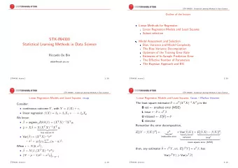
STK-IN4300 - Statistical Learning Methods in Data Science STK-IN4300 - Statistical Learning Methods in Data Science L 2 boosting with linear learner: algorithm L 2 boosting with linear learner: boosting operator Consider a linear regression example, y i “ f p x i q ` ǫ i , i “ 1 , . . . , N, L 2 Boost algorithm: in which: 1. initialize the estimate with least squares, ˆ f 0 p x q “ h p x, ˆ θ y,X q , ‚ ǫ i i.i.d. with E r ǫ i s “ 0 , Var r ǫ i s “ σ 2 ; § ˆ ř N θ y,X “ argmin θ i “ 1 p Y i ´ h p x, θ qq 2 ; ‚ we use a linear learner S : R N Ñ R N ( S y “ ˆ y ); § e.g., S “ νX p X T X q ´ 1 X T . 2. for m “ 1 , . . . , m stop , 2.1 compute the residuals, u m “ y i ´ ˆ f m ´ 1 p x q ; Note that, using an L 2 loss function, 2.2 fit the base learner to the residuals by (regularized, e.g. ν ¨ ) ‚ ˆ f m p x q “ ˆ f m ´ 1 p x q ` S u m ; least squares, h m p x, ˆ θ y,X q ; ‚ u m “ y ´ ˆ f m ´ 1 p x q “ u m ´ 1 ´ S u m ´ 1 “ p I ´ S q u m ´ 1 ; ‚ iterating, u m “ p I ´ S q m , m “ 1 , . . . , m stop . 2.3 update the estimate, f m p x q “ f m ´ 1 p x q ` h m p u m , x q . f m stop p x q “ ř m stop 3. final estimate, ˆ f m stop p x q “ ř m stop m “ 1 h m p u m , x q Because ˆ f m p x q “ S y , then ˆ m “ 0 S p I ´ S q m y , i.e., f m stop p x q “ p I ´ p I ´ S q m ` 1 q ˆ y. looooooooomooooooooon boosting operator B m STK-IN4300: lecture 11 5/ 44 STK-IN4300: lecture 11 6/ 44 STK-IN4300 - Statistical Learning Methods in Data Science STK-IN4300 - Statistical Learning Methods in Data Science L 2 boosting with linear learner: properties L 2 boosting with linear learner: properties We can now compute (B¨ uhlmann & Yu, 2003, Proposition 3): Consider a linear learner S (e.g., least square) with eigenvalues λ k , N k “ 1 , . . . , N . Then ÿ ‚ bias 2 p m, S ; f q “ N ´ 1 p E r ˆ f m p x i qs ´ f q 2 Proposition 2 (B¨ uhlmann & Yu, 2003): The eigenvalues of the i “ 1 L 2 Boost operator B m are “ N ´ 1 f T U diag pp 1 ´ λ k q 2 m ` 2 q U T f ; N 1 ´ p 1 ´ λ k q m stop ` 1 , k “ 1 , . . . , N � ( . ‚ Var p m, S ; σ 2 q “ N ´ 1 ÿ p Var r ˆ f m p x i qsq If S “ S T (i.e., symmetric), then B m can be diagonalized with an i “ 1 N orthonormal transformation, “ σ 2 N ´ 1 ÿ p 1 ´ p 1 ´ λ k q m ` 1 q 2 ; B m “ UD m U T , i “ 1 D m “ diag p 1 ´ p 1 ´ λ k q m stop ` 1 q and where UU T “ U T U “ I . ‚ MSE p m, S ; f, σ 2 q “ bias 2 p m, S ; f q ` Var p m, S ; σ 2 q . STK-IN4300: lecture 11 7/ 44 STK-IN4300: lecture 11 8/ 44
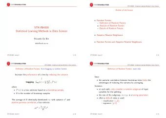
STK-IN4300 - Statistical Learning Methods in Data Science STK-IN4300 - Statistical Learning Methods in Data Science L 2 boosting with linear learner: properties L 2 boosting with linear learner: properties Assuming 0 ă λ k ď 1 , k “ 1 , . . . , N , note that: ‚ bias 2 p m, S ; f q decays exponentially fast for m increasing; ‚ Var p m, S ; σ 2 q increases exponentially slow for m increasing; ‚ lim m Ñ8 MSE p m, S ; f, σ 2 q “ σ 2 ; ‚ if D k : λ k ă 1 (i.e., S ‰ I ), then D m : MSE p m, S ; f, σ 2 q ă σ 2 ; ‚ if @ k : λ k ă 1 , µ 2 1 σ 2 ą p 1 ´ λ k q 2 ´ 1 , then MSE B m ă MSE S , k where µ “ U T f ( µ represents f in the coordinate system of the eigenvectors of S ). (for the proof, see B¨ uhlmann & Yu, 2003, Theorem 1) STK-IN4300: lecture 11 9/ 44 STK-IN4300: lecture 11 10/ 44 STK-IN4300 - Statistical Learning Methods in Data Science STK-IN4300 - Statistical Learning Methods in Data Science L 2 boosting with linear learner: properties L 2 boosting with linear learner: properties There is a further intersting theorem in B¨ uhlmann & Yu (2003), About µ 2 1 σ 2 ą p 1 ´ λ k q 2 ´ 1 : k Theorem 2: Under the assumption seen till here and 0 ă λ k ď 1 , ‚ a large left side means that f is relatively complex compared k “ 1 , . . . , N , and assuming that E r| ǫ 1 | p s ă 8 for p P N , with the noise level σ 2 ; ‚ a small right side means that λ k is small, i.e. the learner N f m p x i q ´ f p x i qq p s “ E r ǫ p shrinks strongly in the direction of the k -th eigenvector; N ´ 1 ÿ E rp ˆ 1 s ` O p e ´ Cm q , m Ñ 8 ‚ therefore, to have boosting bringing improvements: i “ 1 § there must be a large signal to noise ratio; where C ą 0 does not depend on m (but on N and p ). § the value of λ k must be sufficiently small; Ó This theorem can be used to argue that boosting for classification use a weak learner!!! is resistant to overfitting (for m Ñ 8 , exponentially small overfitting). STK-IN4300: lecture 11 11/ 44 STK-IN4300: lecture 11 12/ 44
STK-IN4300 - Statistical Learning Methods in Data Science STK-IN4300 - Statistical Learning Methods in Data Science Gradient Boosting: boosting in high-dimensions Gradient Boosting: component-wise boosting algorithm Component-wise boosting algorithm: f r 0 s 1. initialize the estimate, e.g., ˆ j p x q ” 0 , j “ 1 , . . . , p ; The boosting algorithm is working in high-dimension frameworks: 2. for m “ 1 , . . . , m stop , ‚ forward stagewise additive modelling; § compute the negative gradient vector, ‚ at each step, only one dimension (component) of X is updated ˇ u “ ´ B L p y,f p x qq f r m ´ 1 s p x q ; ˇ at each iteration; B f p x q ˇ f p x q“ ˆ § fit the base learner to the negative gradient vector, ˆ h j p u, x j q , ‚ in a parametric setting, only one ˆ β j is updated; for the j -th component only; ‚ an additional step in which it is decided which component to § select the best update j ˚ (usually that minimizes the loss); update must be computed at each iteration. f r m s f r m ´ 1 s § update the estimate, ˆ j ˚ p x q “ ˆ ` ν ˆ h j ˚ p u, x j ˚ q ; j ˚ § all the other componets do not change. f r m stop s 3. final estimate, ˆ f m stop p x q “ ř p j “ 1 ˆ p x q . j STK-IN4300: lecture 11 13/ 44 STK-IN4300: lecture 11 14/ 44 STK-IN4300 - Statistical Learning Methods in Data Science STK-IN4300 - Statistical Learning Methods in Data Science Gradient Boosting: component-wise boosting with parametric learner Boosting: minimization of the loss function 4 −90 −200 − 2 5 0 −70 Component-wise boosting algorithm with parametric learner: −190 −240 − 5 0 −180 −230 β r 0 s “ p 0 , . . . , 0 q ; −30 1. initialize the estimate, e.g., ˆ −220 −10 −210 3 2. for m “ 1 , . . . , m stop , § compute the negative gradient vector, ˇ u “ ´ B L p y,f p x,β qq β r m ´ 1 s , for the j -th component only; ˇ − B f p x,β q β 2 2 0 2 ˇ β “ ˆ −40 § fit the base learner to the negative gradient vector, ˆ h j p u, x j q ; −60 § select the best update j ˚ (usually that minimizes the loss); −80 −110 −100 −150 − 1 2 0 § include the shrinkage factor, ˆ b j “ ν ˆ −130 h p u, x j q ; −140 1 −180 −160 −170 − −190 β r m s β r m ´ 1 2 1 § update the estimate, ˆ j ˚ “ ˆ ` ˆ 0 b j ˚ . − 2 0 0 − 2 −220 3 0 j ˚ − 2 4 0 −250 β r m stop s (for linear regression). f m stop p x q “ X T ˆ 3. final estimate, ˆ 0 0 1 2 3 4 β 1 STK-IN4300: lecture 11 15/ 44 STK-IN4300: lecture 11 16/ 44
Recommend
More recommend
Explore More Topics
Stay informed with curated content and fresh updates.

