Lecture 10: Neural Networks (Part 2) Feb 25th, 2020 Lecturer: - PDF document

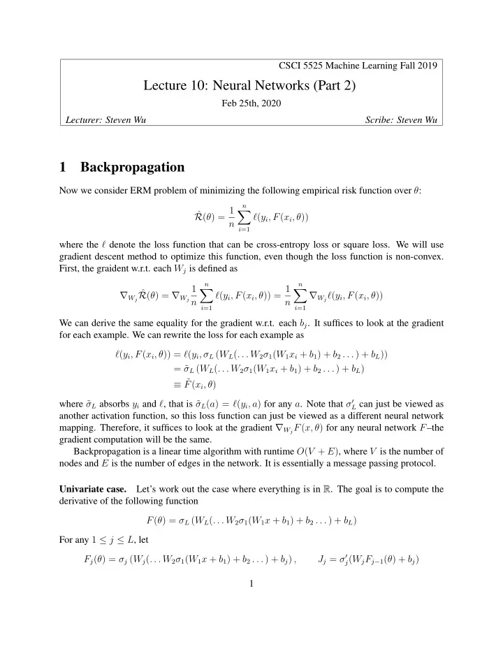
CSCI 5525 Machine Learning Fall 2019 Lecture 10: Neural Networks (Part 2) Feb 25th, 2020 Lecturer: Steven Wu Scribe: Steven Wu 1 Backpropagation Now we consider ERM problem of minimizing the following empirical risk function over θ : n R ( θ ) = 1 ˆ � ℓ ( y i , F ( x i , θ )) n i =1 where the ℓ denote the loss function that can be cross-entropy loss or square loss. We will use gradient descent method to optimize this function, even though the loss function is non-convex. First, the graident w.r.t. each W j is defined as n n 1 ℓ ( y i , F ( x i , θ )) = 1 ∇ W j ˆ � � R ( θ ) = ∇ W j ∇ W j ℓ ( y i , F ( x i , θ )) n n i =1 i =1 We can derive the same equality for the gradient w.r.t. each b j . It suffices to look at the gradient for each example. We can rewrite the loss for each example as ℓ ( y i , F ( x i , θ )) = ℓ ( y i , σ L ( W L ( . . . W 2 σ 1 ( W 1 x i + b 1 ) + b 2 . . . ) + b L )) = ˜ σ L ( W L ( . . . W 2 σ 1 ( W 1 x i + b 1 ) + b 2 . . . ) + b L ) ≡ ˜ F ( x i , θ ) where ˜ σ L absorbs y i and ℓ , that is ˜ σ L ( a ) = ℓ ( y i , a ) for any a . Note that σ ′ L can just be viewed as another activation function, so this loss function can just be viewed as a different neural network mapping. Therefore, it suffices to look at the gradient ∇ W j F ( x, θ ) for any neural network F –the gradient computation will be the same. Backpropagation is a linear time algorithm with runtime O ( V + E ) , where V is the number of nodes and E is the number of edges in the network. It is essentially a message passing protocol. Univariate case. Let’s work out the case where everything is in R . The goal is to compute the derivative of the following function F ( θ ) = σ L ( W L ( . . . W 2 σ 1 ( W 1 x + b 1 ) + b 2 . . . ) + b L ) For any 1 ≤ j ≤ L , let J j = σ ′ F j ( θ ) = σ j ( W j ( . . . W 2 σ 1 ( W 1 x + b 1 ) + b 2 . . . ) + b j ) , j ( W j F j − 1 ( θ ) + b j ) 1

All of these quantities can be computed with a forward pass . Next, we can apply chain rule and compute derivative with a backward pass : ∂F L = J L F L − 1 ( θ ) ∂W L ∂F L = J L ∂b L . . . ∂F L = J L W L J L − 1 W L − 1 . . . F j − 1 ( θ ) ∂W j ∂F L = J L W L J L − 1 W L − 1 . . . J j ∂b j Multivariate case. That looks nice and simple. Now as we move to multi-dimensional case, we will need the following multivariate chain rule: ∇ W f ( Wa ) = J ⊺ a ⊺ where J ∈ R l × R k is the Jacobian matrix of f : R k → R l at Wa . (Recall that for any function f ( r 1 , . . . , r k ) = ( y 1 , . . . y l ) , the entry J ij = ∂y i /∂r j .) Applying chain rule again: ∂F L = J ⊺ L F L − 1 ( θ ) ⊺ ∂W L ∂F L = J ⊺ L ∂b L . . . ∂F L = ( J L W L J L − 1 W L − 1 . . . J j ) ⊺ F j − 1 ( θ ) ⊺ ∂W j ∂F L = ( J L W L J L − 1 W L − 1 . . . J j ) ⊺ ∂b j where J j is the Jacobian of σ j at W j F j − 1 ( θ ) + b j . If σ j is applying the coordinatewise activation function, then the Jacobian matrix is diagonal. 2 Stochastic Gradient Descent Recall that the empirical gradient is defined as n 1 ∇ θ ˆ � R ( θ ) = ∇ θ ℓ ( y i , F ( x i , θ )) n i =1 2

For large n , this can be very expensive to compute. A common practice is to evaluate the gradient i ) } b on a mini-batch { ( x ′ i , y ′ i =1 selected uniformly at random. In expectation, the update is moving to the right direction: � � 1 � = ∇ θ ˆ i , F ( x i , θ t )) R ( θ t ) ∇ θ ℓ ( y ′ E b i The batch size is another hyperparameter to tune. 3