Lecture 10: Classification and Logistic Regression CS109A - PowerPoint PPT Presentation

Lecture 10: Classification and Logistic Regression CS109A Introduction to Data Science Pavlos Protopapas and Kevin Rader

Lecture Outline • Why not Linear Regression? • Binary Response & Logistic Regression • Estimating the Simple Logistic Model • Classification using the Logistic Model • Extending the Logistic Model • Multiple Logistic Regression • Classification Boundaries CS109A, P ROTOPAPAS , R ADER

Advertising Data (from earlier lectures) X Y predictors outcome features response variable covariates dependent variable n observations TV radio newspaper sales 230.1 37.8 69.2 22.1 44.5 39.3 45.1 10.4 17.2 45.9 69.3 9.3 151.5 41.3 58.5 18.5 180.8 10.8 58.4 12.9 p predictors CS109A, P ROTOPAPAS , R ADER 3

Heart Data response variable Y is Yes/No Age Sex ChestPain RestBP Chol Fbs RestECG MaxHR ExAng Oldpeak Slope Ca Thal AHD typical 0.0 fixed 63 1 145 233 1 2 150 0 2.3 3 No asymptomatic 160 3.0 normal 67 1 286 0 2 108 1 1.5 2 Yes 67 1 asymptomatic 120 229 0 2 129 1 2.6 2 2.0 reversable Yes 37 1 nonanginal 130 250 0 0 187 0 3.5 3 0.0 normal No 41 0 nontypical 130 204 0 2 172 0 1.4 1 0.0 normal No CS109A, P ROTOPAPAS , R ADER

Heart Data These data contain a binary outcome HD for 303 patients who presented with chest pain. An outcome value of: • Yes indicates the presence of heart disease based on an angiographic test, • No means no heart disease. There are 13 predictors including: • Age • Sex (0 for women, 1 for men) • Chol (a cholesterol measurement), • MaxHR • RestBP and other heart and lung function measurements. CS109A, P ROTOPAPAS , R ADER

Classification CS109A, P ROTOPAPAS , R ADER

Classification Up to this point, the methods we have seen have centered around modeling and the prediction of a quantitative response variable (ex, number of taxi pickups, number of bike rentals, etc). Linear regression (and Ridge, LASSO, etc) perform well under these situations When the response variable is categorical , then the problem is no longer called a regression problem but is instead labeled as a classification problem . The goal is to attempt to classify each observation into a category (aka, class or cluster) defined by Y , based on a set of predictor variables X . CS109A, P ROTOPAPAS , R ADER

Typical Classification Examples The motivating examples for this lecture(s), homework, and coming labs are based [mostly] on medical data sets. Classification problems are common in this domain: • Trying to determine where to set the cut-off for some diagnostic test (pregnancy tests, prostate or breast cancer screening tests, etc...) • Trying to determine if cancer has gone into remission based on treatment and various other indicators • Trying to classify patients into types or classes of disease based on various genomic markers CS109A, P ROTOPAPAS , R ADER

Why not Linear Regression? CS109A, P ROTOPAPAS , R ADER

Simple Classification Example Given a dataset: { ( x 1 , y 1 ) , ( x 2 , y 2 ) , · · · , ( x N , y N ) } where the 𝑧 are categorical (sometimes referred to as qualitative ), we would like to be able to predict which category 𝑧 takes on given 𝑦 . Linear regression does not work well , or is not appropriate at all, in this setting. A categorical variable 𝑧 could be encoded to be quantitative. For example, if 𝑧 represents concentration of Harvard undergrads, then 𝑧 could take on the values:  1 if Computer Science (CS)  2 if Statistics y = . 3 otherwise  CS109A, P ROTOPAPAS , R ADER

Simple Classification Example A linear regression could be used to predict y from x . What would be wrong with such a model? The model would imply a specific ordering of the outcome, and would treat a one-unit change in y equivalent. The jump from y =1 to y=2 (CS to Statistics) should not be interpreted as the same as a jump from y =2 to y =3 (Statistics to everyone else). Similarly, the response variable could be reordered such that y =1 represents Statistics and y =2 represents CS, and then the model estimates and predictions would be fundamentally different. If the categorical response variable was ordinal (had a natural ordering, like class year, Freshman, Sophomore, etc.), then a linear regression model would make some sense but is still not ideal. CS109A, P ROTOPAPAS , R ADER

Even Simpler Classification Problem: Binary Response The simplest form of classification is when the response variable 𝑍 has only two categories, and then an ordering of the categories is natural. For example, an upperclassmen Harvard student could be categorized as (note, the 𝑧 =0 category is a "catch-all" so it would involve both River House students and those who live in other situations: off campus, etc): ⇢ 1 if lives in the Quad y = . 0 otherwise Linear regression could be used to predict 𝑧 directly from a set of covariates (like sex, whether an athlete or not, concentration, GPA, etc.), and if ​𝑧 ≥0.5, we could predict the student lives in the Quad and predict other houses if ​𝑧 <0.5 . CS109A, P ROTOPAPAS , R ADER

Even Simpler Classification Problem: Binary Response What could go wrong with this linear regression model? . CS109A, P ROTOPAPAS , R ADER

Even Simpler Classification Problem: Binary Response The main issue is you could get non-sensical values for 𝑧 . Since this is modeling 𝑄 ( 𝑧 =1) , values for ​𝑧 below 0 and above 1 would be at odds with the natural measure for 𝑧 . Linear regression can lead to this issue. CS109A, P ROTOPAPAS , R ADER

Binary Response & Logistic Regression CS109A, P ROTOPAPAS , R ADER

Pavlos Game #45 Think of a function that would do this for us 𝑍 = 𝑔 ( 𝑦 ) CS109A, P ROTOPAPAS , R ADER

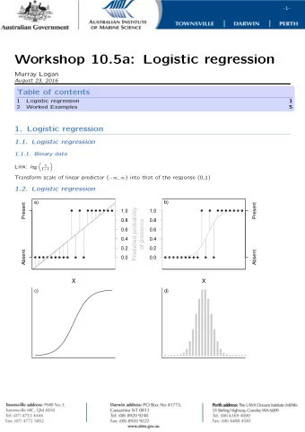
Logistic Regression Logistic Regression addresses the problem of estimating a probability, 𝑄(𝑧 =1 ) , to be outside the range of [0,1] . The logistic regression model uses a function, called the logistic function, to model 𝑄(𝑧 =1 ) : e β 0 + β 1 X 1 P ( Y = 1) = 1 + e β 0 + β 1 X = 1 + e − ( β 0 + β 1 X ) CS109A, P ROTOPAPAS , R ADER

Logistic Regression As a result the model will predict 𝑄(𝑧 =1 ) with an 𝑇 -shaped curve, which is the general shape of the logistic function. ​𝛾↓ 0 shifts the curve right or left. ​𝛾↓ 1 controls how steep the 𝑇 -shaped curve is. Note: if ​𝛾↓ 1 is positive, then the predicted 𝑄(𝑧 =1 ) goes from zero for small values of 𝑌 to one for large values of 𝑌 and if ​𝛾↓ 1 is negative, then has the 𝑄(𝑧 =1 ) opposite association. CS109A, P ROTOPAPAS , R ADER

Logistic Regression 1 P ( Y = 1) = 1 + e − ( β 0 + β 1 X ) CS109A, P ROTOPAPAS , R ADER

Logistic Regression 1 P ( Y = 1) = 1 + e − ( β 0 + β 1 X ) CS109A, P ROTOPAPAS , R ADER

Logistic Regression With a little bit of algebraic work, the logistic model can be rewritten as: ✓ P ( Y = 1) ◆ ln = β 0 + β 1 X. 1 − P ( Y = 1) The value inside the natural log function ​𝑄 ( 𝑍 =1) / 1− 𝑄 ( 𝑍 =1) , is called the odds , thus logistic regression is said to model the log-odds with a linear function of the predictors or features, 𝑌 . This gives us the natural interpretation of the estimates similar to linear regression: a one unit change in 𝑌 is associated with a ​𝛾↓ 1 change in the log-odds of 𝑍 =1 ; or better yet, a one unit change in 𝑌 is associated with an ​𝑓↑​𝛾↓ 1 change in the odds that 𝑍 =1 . CS109A, P ROTOPAPAS , R ADER

Estimating the Simple Logistic Model CS109A, P ROTOPAPAS , R ADER

Estimation in Logistic Regression Unlike in linear regression where there exists a closed-form solution to finding the estimates, ​𝛾 ↓𝑘 ’s, for the true parameters, logistic regression estimates cannot be calculated through simple matrix multiplication. In linear regression what loss function was used to determine the parameter estimates? What was the probabilistic perspective on linear regression? Logistic Regression also has a likelihood based approach to estimating parameter coefficients. CS109A, P ROTOPAPAS , R ADER

Estimation in Logistic Regression Probability: 𝑍 =1: 𝑞 Probability: 𝑍 =0:1− 𝑞 ​𝑄(𝑍 = 𝑧) = 𝑞↑𝑧 ​ (1− 𝑞 ) ↑ (1− 𝑧 ) Where: 𝑞 = 𝑄 ( 𝑍 =1| 𝑌 = 𝑦 ) and therefore p depends on X. Thus not every p is the same for each individual measurement. CS109A, P ROTOPAPAS , R ADER

Likelihood The likelihood of a single observation for p given x and y is: L ( p i | Y i ) = P ( Y i = y i ) = p y i i (1 − p ) 1 − y i Given the observations are independent, what is the likelihood function for p ? Y Y p y i i (1 − p ) 1 − y i L ( p | Y ) = P ( Y i = y i ) = i i ◆ y i ✓ ◆ 1 − y i e X i β e X i β ✓ Y L ( p | Y ) = 1 − 1 + e X i β 1 + e X i β i CS109A, P ROTOPAPAS , R ADER

Likelihood ◆ y i ✓ ◆ 1 − y i e X i β e X i β ✓ Y L ( p | Y ) = 1 − 1 + e X i β 1 + e X i β i How do we maximize this? Take the log and differentiate! But jeeze does this look messy?! It will not necessarily have a closed form solution? So how do we determine the parameter estimates? Through an iterative approach (we will talk more about it next lecture). CS109A, P ROTOPAPAS , R ADER