Learning Summary Given a task, use data/experience bias/background - PowerPoint PPT Presentation

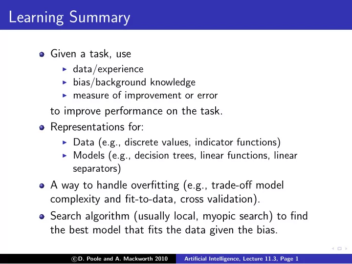
Learning Summary Given a task, use ◮ data/experience ◮ bias/background knowledge ◮ measure of improvement or error to improve performance on the task. Representations for: ◮ Data (e.g., discrete values, indicator functions) ◮ Models (e.g., decision trees, linear functions, linear separators) A way to handle overfitting (e.g., trade-off model complexity and fit-to-data, cross validation). Search algorithm (usually local, myopic search) to find the best model that fits the data given the bias. � D. Poole and A. Mackworth 2010 c Artificial Intelligence, Lecture 11.3, Page 1

Learning Objectives - Reinforcement Learning At the end of the class you should be able to: Explain the relationship between decision-theoretic planning (MDPs) and reinforcement learning Implement basic state-based reinforcement learning algorithms: Q-learning and SARSA Explain the explore-exploit dilemma and solutions Explain the difference between on-policy and off-policy reinforcement learning � D. Poole and A. Mackworth 2010 c Artificial Intelligence, Lecture 11.3, Page 2

Reinforcement Learning What should an agent do given: Prior knowledge possible states of the world possible actions Observations current state of world immediate reward / punishment Goal act to maximize accumulated (discounted) reward Like decision-theoretic planning, except model of dynamics and model of reward not given. � D. Poole and A. Mackworth 2010 c Artificial Intelligence, Lecture 11.3, Page 3

Reinforcement Learning Examples Game - reward winning, punish losing Dog - reward obedience, punish destructive behavior Robot - reward task completion, punish dangerous behavior � D. Poole and A. Mackworth 2010 c Artificial Intelligence, Lecture 11.3, Page 4

Experiences We assume there is a sequence of experiences: state , action , reward , state , action , reward , .... At any time it must decide whether to explore to gain more knowledge ◮ exploit knowledge it has already discovered ◮ � D. Poole and A. Mackworth 2010 c Artificial Intelligence, Lecture 11.3, Page 5

Why is reinforcement learning hard? What actions are responsible for a reward may have occurred a long time before the reward was received. The long-term effect of an action depend on what the agent will do in the future. The explore-exploit dilemma: at each time should the agent be greedy or inquisitive? � D. Poole and A. Mackworth 2010 c Artificial Intelligence, Lecture 11.3, Page 6

Reinforcement learning: main approaches search through a space of policies (controllers) learn a model consisting of state transition function P ( s ′ | a , s ) and reward function R ( s , a , s ′ ); solve this an an MDP. learn Q ∗ ( s , a ), use this to guide action. � D. Poole and A. Mackworth 2010 c Artificial Intelligence, Lecture 11.3, Page 7

Recall: Asynchronous VI for MDPs, storing Q [ s , a ] (If we knew the model:) Initialize Q [ S , A ] arbitrarily Repeat forever: Select state s , action a � � � Q [ s , a ] ← P ( s ′ | s , a ) R ( s , a , s ′ ) + γ max a ′ Q [ s ′ , a ′ ] s ′ � D. Poole and A. Mackworth 2010 c Artificial Intelligence, Lecture 11.3, Page 8

Reinforcement Learning (Deterministic case) flat or modular or hierarchical explicit states or features or individuals and relations static or finite stage or indefinite stage or infinite stage fully observable or partially observable deterministic or stochastic dynamics goals or complex preferences single agent or multiple agents knowledge is given or knowledge is learned perfect rationality or bounded rationality � D. Poole and A. Mackworth 2010 c Artificial Intelligence, Lecture 11.3, Page 9

Experiential Asynchronous Value Iteration for Deterministic RL initialize Q [ S , A ] arbitrarily observe current state s repeat forever: select and carry out an action a observe reward r and state s ′ What do we know now? � D. Poole and A. Mackworth 2010 c Artificial Intelligence, Lecture 11.3, Page 10

Experiential Asynchronous Value Iteration for Deterministic RL initialize Q [ S , A ] arbitrarily observe current state s repeat forever: select and carry out an action a observe reward r and state s ′ Q [ s , a ] ← r + γ max a ′ Q [ s ′ , a ′ ] s ← s ′ � D. Poole and A. Mackworth 2010 c Artificial Intelligence, Lecture 11.3, Page 11

Reinforcement Learning flat or modular or hierarchical explicit states or features or individuals and relations static or finite stage or indefinite stage or infinite stage fully observable or partially observable deterministic or stochastic dynamics goals or complex preferences single agent or multiple agents knowledge is given or knowledge is learned perfect rationality or bounded rationality � D. Poole and A. Mackworth 2010 c Artificial Intelligence, Lecture 11.3, Page 12

Temporal Differences Suppose we have a sequence of values: v 1 , v 2 , v 3 , . . . and want a running estimate of the average of the first k values: A k = v 1 + · · · + v k k � D. Poole and A. Mackworth 2010 c Artificial Intelligence, Lecture 11.3, Page 13

Temporal Differences (cont) Suppose we know A k − 1 and a new value v k arrives: v 1 + · · · + v k − 1 + v k A k = k = � D. Poole and A. Mackworth 2010 c Artificial Intelligence, Lecture 11.3, Page 14

Temporal Differences (cont) Suppose we know A k − 1 and a new value v k arrives: v 1 + · · · + v k − 1 + v k A k = k k − 1 A k − 1 + 1 = k v k k Let α k = 1 k , then = A k � D. Poole and A. Mackworth 2010 c Artificial Intelligence, Lecture 11.3, Page 15

Temporal Differences (cont) Suppose we know A k − 1 and a new value v k arrives: v 1 + · · · + v k − 1 + v k A k = k k − 1 A k − 1 + 1 = k v k k Let α k = 1 k , then = (1 − α k ) A k − 1 + α k v k A k = A k − 1 + α k ( v k − A k − 1 ) “TD formula” Often we use this update with α fixed. We can guarantee convergence to average if ∞ ∞ � � α 2 α k = ∞ and k < ∞ . k =1 k =1 � D. Poole and A. Mackworth 2010 c Artificial Intelligence, Lecture 11.3, Page 16

Q-learning Idea: store Q [ State , Action ]; update this as in asynchronous value iteration, but using experience (empirical probabilities and rewards). Suppose the agent has an experience � s , a , r , s ′ � This provides one piece of data to update Q [ s , a ]. An experience � s , a , r , s ′ � provides a new estimate for the value of Q ∗ ( s , a ): which can be used in the TD formula giving: � D. Poole and A. Mackworth 2010 c Artificial Intelligence, Lecture 11.3, Page 17

Q-learning Idea: store Q [ State , Action ]; update this as in asynchronous value iteration, but using experience (empirical probabilities and rewards). Suppose the agent has an experience � s , a , r , s ′ � This provides one piece of data to update Q [ s , a ]. An experience � s , a , r , s ′ � provides a new estimate for the value of Q ∗ ( s , a ): r + γ max a ′ Q [ s ′ , a ′ ] which can be used in the TD formula giving: � D. Poole and A. Mackworth 2010 c Artificial Intelligence, Lecture 11.3, Page 18

Q-learning Idea: store Q [ State , Action ]; update this as in asynchronous value iteration, but using experience (empirical probabilities and rewards). Suppose the agent has an experience � s , a , r , s ′ � This provides one piece of data to update Q [ s , a ]. An experience � s , a , r , s ′ � provides a new estimate for the value of Q ∗ ( s , a ): r + γ max a ′ Q [ s ′ , a ′ ] which can be used in the TD formula giving: � � a ′ Q [ s ′ , a ′ ] − Q [ s , a ] Q [ s , a ] ← Q [ s , a ] + α r + γ max � D. Poole and A. Mackworth 2010 c Artificial Intelligence, Lecture 11.3, Page 19

Q-learning initialize Q [ S , A ] arbitrarily observe current state s repeat forever: select and carry out an action a observe reward r and state s ′ Q [ s , a ] ← Q [ s , a ] + α ( r + γ max a ′ Q [ s ′ , a ′ ] − Q [ s , a ]) s ← s ′ � D. Poole and A. Mackworth 2010 c Artificial Intelligence, Lecture 11.3, Page 20

Properties of Q-learning Q-learning converges to an optimal policy, no matter what the agent does, as long as it tries each action in each state enough. But what should the agent do? ◮ exploit: when in state s , ◮ explore: � D. Poole and A. Mackworth 2010 c Artificial Intelligence, Lecture 11.3, Page 21

Properties of Q-learning Q-learning converges to an optimal policy, no matter what the agent does, as long as it tries each action in each state enough. But what should the agent do? ◮ exploit: when in state s , select an action that maximizes Q [ s , a ] ◮ explore: select another action � D. Poole and A. Mackworth 2010 c Artificial Intelligence, Lecture 11.3, Page 22

Exploration Strategies The ǫ -greedy strategy: choose a random action with probability ǫ and choose a best action with probability 1 − ǫ . � D. Poole and A. Mackworth 2010 c Artificial Intelligence, Lecture 11.3, Page 23

Exploration Strategies The ǫ -greedy strategy: choose a random action with probability ǫ and choose a best action with probability 1 − ǫ . Softmax action selection: in state s , choose action a with probability e Q [ s , a ] /τ � a e Q [ s , a ] /τ where τ > 0 is the temperature . Good actions are chosen more often than bad actions. τ defines how much a difference in Q-values maps to a difference in probability. � D. Poole and A. Mackworth 2010 c Artificial Intelligence, Lecture 11.3, Page 24