LEARNING Master in Artificial Intelligence Reference Christopher - PowerPoint PPT Presentation
SYMBOLIC and STATISTICAL LEARNING Master in Artificial Intelligence Reference Christopher M. Bishop - Pattern Recognition and Machine Learning, Chapter 1 & 2 The Gaussian Distribution Gaussian Mean and Variance Maximum Likelihood Use
SYMBOLIC and STATISTICAL LEARNING Master in Artificial Intelligence
Reference Christopher M. Bishop - Pattern Recognition and Machine Learning, Chapter 1 & 2
The Gaussian Distribution
Gaussian Mean and Variance
Maximum Likelihood Use the training data { x , t } to determine the values of the unknown parameters w and β by maximum likelihood. Maximizing likelihood is equivalent, so far as determining w is concerned, to minimizing the sum-of-squares error function. Determine by minimizing sum-of-squares error, .
Predictive Distribution
MAP: A Step towards Bayes Determine by minimizing regularized sum-of-squares error, .
Bayesian Curve Fitting
Bayesian Predictive Distribution
Model Selection What’s the best model complexity that give the best generalization? (M, λ ) If enough data: - Parts of them are used for training a range of models - Parts are used as validation data to detect the best model - Parts are kept for the test set for evaluation Limited data we wish to use most of it for training small validation set noisy estimation of predictive performance
Cross-Validation Main disadvantages: - no of runs is increased by a factor of S - Multiple complexity parameters for the same model (ex: λ ) If no of partitions (S) = no of training instances leave-one-out
Curse of Dimensionality – Example (1) Problem: 12-dimensional reprezentation of some points, only 2 dimension presented in the diagram How should be classified the point represented by a cross: blue, red or green?
Curse of Dimensionality – Example (2) Divide the space and assign the division the class represented by the majority of points What happens when the space is multi- dimensional? Think of these two squares …
Curse of Dimensionality We have to add 10 dimensions, what will happen with the squares indicated by arrows? – exponential number of n-dimensional spaces Where do we get the training data for the exponential spaces that are obtained?
Curse of Dimensionality Go back to the curve fitting problem and addapt it: Polynomial curve fitting, M = 3 A no ∝ D M of coeficients have to be computed – power grow instead of exponential
Curse of Dimensionality Properties that can be exploited: - Real data is confined to a space having lower dimensionality and the directions over which important variations in the target variables occur may be so confined - real data will typically exhibit some smoothness properties (at least locally) so that for Gaussian Densities in the most part small changes higher dimensions in the input variables will produce small changes in the In high dimensional spaces, the target variables, so they can probability mass of the be determined using Gaussian is concentrated in a interpolation techniques thin shell
Decision Theory Probability theory – how to deal with uncertainty Decision theory – combined with probability theory helps us to make optimal decisions in situations involving uncertainty Inference step Determine either or . Decision step For given x , determine optimal t .
Decision Theory - Example Problem: Cancer diagnosis based on an X-ray image of a patient Input: a vector x of the pixels intensities of the image Ouput: has cancer or not (binary output) Inference step: determine p(x, cancer); p(x, not_cancer) Decision step: Patient has cancer or not
Minimum Misclassification Rate Goal: assign each value of x to a class so to make as few misclassifications as possible Space is divided in decision regions R k – the limits – decision boundaries / surfaces p(x, C k ) = p( C k |x) * p(x) X assigned to the class that has max p( C k |x)
Minimum Expected Loss Example: classify medical images as ‘cancer’ or ‘normal’ Much worse to diagnose a sick patient as being well than opposite loss / cost function (utility function) minimize maximize Decision loss matrix Truth If a new value x from the true class C k is assign to class C j we add some loss denoted by L kj in the loss matrix
Minimum Expected Loss We have to minimize the loss function – depends on the true class (unkonwn) The purpose is to minimize the average loss: Regions are chosen to minimize
Reject Option Classification errors arrise from regions where P( x , C k ) have comparable values In such areas we can avoid making decisions in order to lower error rate θ =1 , all examples are rejected, θ < 1/k nothing is rejected
Inference and decision • Alternatives: • Generative models – determine p( x | C k ) or p( x,C k ), derives p( C k ,x ) and make the decision • Advantage: we know p( x ) and can determine new data points • Disadvantage: lots of computation, demands a lot of data • Discriminative models – determine directly p( C k ,x ) and make the decision • Advantage: faster, less demanding (resources, data) • solve both problems by learning a function that maps inputs x directly into decisions – discriminant function • Advantage: simpler method • Disadvantage : we don’t have the probabilities
Why Separate Inference and Decision? • Minimizing risk (loss matrix may change over time) • Reject option (cannot have this option with discriminant functions) • Unbalanced class priors (cancer 0.1% population – training classify all as healthy we need balanced training data and need to compensate the altering of this data by adding the prior probabilities) • Combining models (divide et impera for complex applications – blood tests & X-rays for detecting cancer)
Decision Theory for Regression Inference step Determine . Decision step For given x , make optimal prediction, y ( x ) , for t . Loss function:
The Squared Loss Function ∂ x Noise generated by the training data - min value of the loss function
Generative vs Discriminative Generative approach: Model Use Bayes’ theorem Discriminative approach: Model directly Find a regression function y(x) directly from the training data
Entropy Coding theory: x discrete with 8 possible states; how many bits to transmit the state of x ? All states equally likely (p( x ) = 1/8)
Entropy
Entropy In how many ways can N identical objects be allocated M bins? Entropy maximized when
Entropy
Differential Entropy Put bins of width ¢ along the real line Differential entropy maximized (for fixed ) when in which case
Conditional Entropy
The Kullback-Leibler Divergence KL divergence = measure of dissimilarity between 2 distribution p, and q KL divergence (KL(p ‖ q)) represents the minimum value of the average addition of information that has to be sent when encoding a message x having the distribution p using the distribution q p(x) - unknown q(x| θ )- approximates p(x) x n observed training points drawn from p(x) θ - can be determined by minimizing KL(p ‖ q)
Mutual Information Consider the joint distribution of 2 variables x and y p(x,y): - if x and y are independent: p(x,y)= p(x)*p(y), - if not, we can use K-L divergence to see how closely related they are: I[x,y] (mutual information between x and y) = the reduction in uncertainty about x as a consequence of the new observation y I[x,y] ≥ 0 , I[x,y] = 0 if and only if x and y are independent
SYMBOLIC and STATISTICAL LEARNING Chapter 2: Probability distributions
Basic Notions The role of distribution is to model the probability distribution p(x) density estimation 2 types of distributions: Parametric: - Governed by a small number of adaptive parameters - Ex: binomial, multinomial, Gauss - Try to determine the parameters from the samples - Limitation: assumes a specific functional form for the distribution Nonparametric: - The form of the distribution depends on the size of the data set. - There are parameters, but they control the model complexity rather than the form of the distribution. - Ex: histograms, nearest-neighbours, and kernels.
Binary Variables (1) x ∊ {0, 1} - describes the outcome of a coin flipping: heads = 1, tails = 0 The probability distribution over x is given by the Bernoulli Distribution:
Binary Variables (2) N coin flips: Binomial Distribution
Binomial Distribution
Beta Distribution (I) Distribution over . Γ (x+1) = x Γ (x) = x!
Beta Distribution (II)
The Gaussian Distribution
Central Limit Theorem The distribution of the sum of N i.i.d. random variables becomes increasingly Gaussian as N grows. Example: N uniform [0,1] random variables.
Student’s t -Distribution where Infinite mixture of Gaussians.
Student’s t -Distribution
Periodic variables • Examples: calendar time, direction, … • We require
von Mises Distribution (I) This requirement is satisfied by where
von Mises Distribution (II)
The Exponential Family (1) where η is the natural parameter and so g ( η ) can be interpreted as a normalization coefficient.
The Exponential Family (2.1) The Bernoulli Distribution Comparing with the general form we see that and so Logistic sigmoid
Recommend
More recommend
Explore More Topics
Stay informed with curated content and fresh updates.
