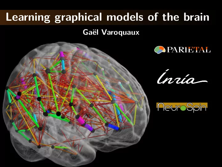
Learning graphical models of the brain Ga el Varoquaux functional - PowerPoint PPT Presentation

Learning graphical models of the brain Ga¨ el Varoquaux

functional MRI (fMRI) t Recordings of brain activity G Varoquaux 2

functional MRI (fMRI) t Recordings of brain activity Brain mapping : the motor system: “move the right hand” the language system: “say three names of animals” G Varoquaux 2

functional MRI (fMRI) Brain mapping : The language network the language system: “say three names of animals” G Varoquaux 3

functional MRI (fMRI) Brain mapping : The language network Interacting sub-systems : Sounds Lexical access Syntax the language system: “say three names of animals” G Varoquaux 3

The functional connectome View of the brain as a set of regions and their interactions G Varoquaux 4

The functional connectome View of the brain as a set of regions and their interactions Intrinsic brain architecture Biomarkers of pathologies Learn a graphical model Human Connectome Project: 30M$ G Varoquaux 4

Resting-state fMRI G Varoquaux 5

Outline 1 Graphical structures of brain activity 2 Multi-subject graph learning 3 Beyond ℓ 1 models G Varoquaux 6

1 Graphical structures of brain activity Functional connectome Graph of interactions between regions [Varoquaux & Craddock 2013] G Varoquaux 7

1 From correlations to connectomes Conditional independence structure? G Varoquaux 8

1 Probabilistic model for interactions Simplest data generating process = multivariate normal: 2 X T Σ − 1 X | Σ − 1 | e − 1 � P ( X ) ∝ Model parametrized by inverse covariance matrix, K = Σ − 1 : conditional covariances Goodness of fit: likelihood of observed covariance ˆ Σ in model Σ L ( ˆ Σ | K ) = log | K | − trace ( ˆ Σ K ) G Varoquaux 9

1 Graphical structure from correlations Observations Direct connections Covariance Inverse covariance 1 1 2 2 0 0 3 3 4 4 Diagonal: Diagonal: signal variance node innovation G Varoquaux 10

1 Independence structure (Markov graph) Zeros in partial correlations give conditional independence Reflects the large-scale brain interaction structure G Varoquaux 11

1 Independence structure (Markov graph) Zeros in partial correlations give conditional independence Ill-posed problem: multi-collinearity ⇒ noisy partial correlations Independence between nodes makes estimation of partial correlations well-conditionned. Chicken and egg problem G Varoquaux 11

1 Independence structure (Markov graph) Zeros in partial correlations give conditional independence Ill-posed problem: multi-collinearity ⇒ noisy partial correlations Independence between nodes makes estimation of partial correlations well-conditionned. 1 1 Joint estimation: 2 2 Sparse inverse covariance + 0 0 3 3 4 4 G Varoquaux 11

1 Sparse inverse covariance estimation: penalized Maximum a posteriori: Fit models with a penalty Sparsity ⇒ Lasso-like problem: ℓ 1 penalization K ≻ 0 L ( ˆ x 2 K = argmin Σ | K ) + λ ℓ 1 ( K ) Data fit, Penalization, x 1 Likelihood [Varoquaux NIPS 2010] [Smith 2011] G Varoquaux 12

x 2 x 1 1 Sparse inverse covariance estimation: penalized Maximum a posteriori: Fit models with a penalty Sparsity ⇒ Lasso-like problem: ℓ 1 penalization K ≻ 0 L ( ˆ K = argmin Σ | K ) + λ ℓ 1 ( K ) Test-data likelihood Optimal graph almost dense Sparsity 2.5 3.0 3.5 4.0 − log 10 λ G Varoquaux 12

x 2 x 1 1 Sparse inverse covariance estimation: penalized Maximum a posteriori: Bias of ℓ 1 : Fit models with a penalty very sparse graphs don’t fit the data Sparsity ⇒ Lasso-like problem: ℓ 1 penalization K ≻ 0 L ( ˆ K = argmin Σ | K ) + λ ℓ 1 ( K ) Test-data likelihood Optimal graph almost dense Sparsity 2.5 3.0 3.5 4.0 − log 10 λ G Varoquaux 12

x 2 x 1 1 Sparse inverse covariance estimation: penalized Maximum a posteriori: Bias of ℓ 1 : Fit models with a penalty very sparse graphs don’t fit the data Sparsity ⇒ Lasso-like problem: ℓ 1 penalization Algorithmic considerations: K ≻ 0 L ( ˆ K = argmin Σ | K ) + λ ℓ 1 ( K ) Very ill-conditionned input matrices Graph-lasso [Friedman 2008] doesn’t work well Test-data likelihood primal-dual algorithm with approximation when switching from dual to primal [Mazumder, 2012] Optimal graph Good success with ADMM almost dense split optimization: loss solved with SPD matrices Sparsity penalty solved with sparse matrices 2.5 3.0 3.5 4.0 − log 10 λ G Varoquaux 12

1 Very sparse graphs: greedy construction Sparse inverse covariance algorithm: PC-DAG [Rutimann & Buhlmann 2009] Greedy approach 1. PC-alg : fill graph by independence tests conditioning on neighbors 2. Learn covariance on resulting structure Good for very sparse graphs [Varoquaux J. Physio Paris, 2012] G Varoquaux 13

1 Sparse graphs: greedy construction Test data likelihood Iterate construction alg. High-degree nodes appear very quickly complexity ∝ exp degree 0 20 Fillingfactor (percents) Lattice-like structure with hubs [Varoquaux J. Physio Paris, 2012] G Varoquaux 14

2 Multi-subject graph learning Not enough data per subject to recover structure G Varoquaux 15

2 Subject-level data scarsity Sparse recovery for Gaussian graphs ℓ 1 structure recovery has phase-transitions behaviors For Gaussian graphs with s edges, p nodes: � √ p � � � n = O ( s + p ) log p s = o , [Lam & Fan 2009] Need to accumulate data across subjects Concatenate series = iid data G Varoquaux 16

2 Graphs on group data ˆ Sparse Sparse group Σ − 1 inverse concat Likelihood of new data (cross-validation) Subject data, Σ − 1 -57.1 Subject data, sparse inverse 43.0 Group concat data, Σ − 1 40.6 Group concat data, sparse inverse 41.8 Inter-subect variability [Varoquaux NIPS 2010] G Varoquaux 17

2 Multi-subject modeling Common independence structure but different connection values s L ( ˆ { K s } = argmin Σ s | K s ) + λ ℓ 21 ( { K s } ) � { K s ≻ 0 } Multi-subject data fit, Group-lasso penalization Likelihood [Varoquaux NIPS 2010] G Varoquaux 18

2 Multi-subject modeling Common independence structure but different connection values s L ( ˆ { K s } = argmin Σ s | K s ) + λ ℓ 21 ( { K s } ) � { K s ≻ 0 } Multi-subject data fit, ℓ 1 on the connections of Likelihood the ℓ 2 on the subjects [Varoquaux NIPS 2010] G Varoquaux 18

2 Population-sparse graph perform better ˆ Population Sparse Σ − 1 prior inverse Likelihood of new data (cross-validation) sparsity Subject data, Σ − 1 -57.1 Subject data, sparse inverse 43.0 60% full Group concat data, Σ − 1 40.6 Group concat data, sparse inverse 41.8 80% full Group sparse model 45.6 20% full [Varoquaux NIPS 2010] G Varoquaux 19

2 Independence structure of brain activity Subject-sparse estimate G Varoquaux 20

2 Independence structure of brain activity Population- sparse estimate G Varoquaux 20

2 Large scale organization High-level cognitive function arises from the interplay of specialized brain regions: The functional segregation of local areas [...] contrasts sharply with their global integration during perception and behavior [Tononi 1994] Functional segregation : nodes of connectome atomic functions – tonotopy Global integration : functional networks high-level functions – language G Varoquaux 21

2 Large scale organization High-level cognitive function arises from the interplay of specialized brain regions: The functional segregation of local areas [...] contrasts sharply with their global integration during perception and behavior [Tononi 1994] Scale-free hierarchical integration / segregation Graph modularity = divide in communities to maximize intra-class connections versus extra-class [Eguiluz 2005] G Varoquaux 21

2 Graph cuts to isolate functional communities Find communities to maximize modularity: 2     k  A ( V c , V c )  A ( V , V c ) Q = � A ( V , V ) −   A ( V , V ) c = 1 A ( V a , V b ) : sum of edges going from V a to V b Rewrite as an eigenvalue problem [White 2005] 1 1 A · 1 1 0 0 0 0 ⇒ Spectral clustering = spectral embedding + k-means Similar to normalized graph cuts G Varoquaux 22

2 Large scale organization Non-sparse Neural communities G Varoquaux 23

2 Large scale organization Group-sparse Neural communities = large known functional networks G Varoquaux 23

2 Brain integration between communities Proposed measure for functional integration: mutual information (Tononi) [Marrelec 2008, Varoquaux & Craddock 2013] Integration: I c 1 = 1 2 log det ( K c 1 ) “energy” in network Mutual information: M c 1 , c 2 = I c 1 ∪ c 2 − I c 1 − I s 2 “cross-talks” between networks G Varoquaux 24

2 Brain integration between communities With population prior: Occipital pole visual areas Default mode network M edial visual areas Fronto-parietal Lateral visual networks areas Fronto-lateral Posterior inferior network temporal 1 Pars Posterior inferior opercularis temporal 2 Right T halamus Dorsal motor Raw Cingulo-insular Ventral motor correlations: network Left Putamen Auditory Basal ganglia [Varoquaux NIPS 2010] G Varoquaux 24

3 Beyond ℓ 1 models Test-data likelihood Sparsity 2.5 3.0 3.5 4.0 − log 10 λ G Varoquaux 25