Learning and Meta-learning computation making predictions choosing - - PDF document

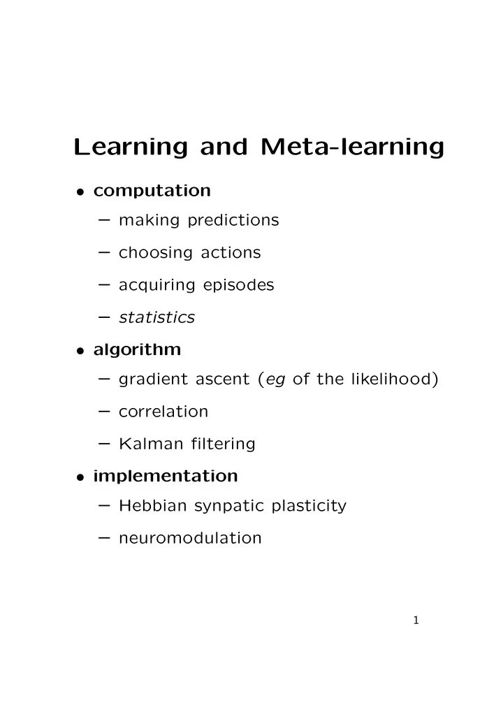
Learning and Meta-learning

• computation

– making predictions – choosing actions – acquiring episodes – statistics

• algorithm

– gradient ascent (eg of the likelihood) – correlation – Kalman filtering

• implementation

– Hebbian synpatic plasticity – neuromodulation

1

Types of Learning

supervised

v|u

inputs u and desired

• r target
• utputs v

both provided, eg prediction→outcome reinforce max r|u input u and scalar evaluation r

• ften with temporal

credit assignment problem unsupervised

u

• r self-supervised

learn structure from statistics These are closely related: supervised learn P[v|u] unsupervised learn P[v, u]

2

Hebb

Famously suggested: if cell A consistently contributes to the activity of cell B, then the synapse from A to B should be strengthened

• strong element of causality
• what about weakening (LTD)?
• multiple timescales – STP to protein

synthesis

• multiple biochemical mechanisms
• systems:

– hippocampus – multiple sub-areas – neocortex – layer and area differences – cerebellum – LTD is the norm

3

Neural Rules

0.1 0.2 0.3 0.4

1 100 s Hz 10 2 min Hz

field potential amplitude (mV) time (min)

10 20 30 40

LTP LTD control level depressed, partially depotentiated level potentiated level

4

Stability and Competition

Hebbian learning involves positive feedback. Control by: LTD usually not enough – covariance versus correlation saturation prevent synaptic weights from getting too big (or too small) – triviality beckons competition spike-time dependent learning rules normalization over pre-synaptic or post-synaptic arbors

• subtractive: decrease all synapses by

the same amount whether large or small

• multiplicative: decrease large synapses

by more than small synapses

5

Preamble

Linear firing rate model τr dv dt = −v + w · u = −v +

Nu

• b=1

wbub assume that τr is small compared with the rate of change of the weights, then v = w · u during plasticity Then have τw dw dt = f(v, u, w) Supervised rules use targets to specify v – neural basis in ACh?

6

The Basic Hebb Rule

τw dw dt = uv averaged over input statistics gives τw dw dt = uv = uu · w = Q · w where Q is the input correlation matrix. Positive feedback instability τw d dt|w|2 = 2τww · dw dt = 2v2 Also have discretised version

w → w + T

τw

Q · w .

integrating over time, presenting patterns for T seconds.

7

Covariance Rule

Since LTD really exists, contra Hebb: τw dw dt =

u

(v − θv)

• r

τw dw dt = (u − θ θ θu) v If θv = v or θ θ θu = u then τw dw dt = C · w where C = (u − u)(u − u) is the input covariance matrix. Still unstable τw d dt|w|2 = 2v(v − v) which averages to the (positive) covariance of v.

8

BCM Rule

Odd to have LTD with v = 0 or u = 0 0. Evidence for τw dw dt = vu (v − θv) .

0.5 1 1.5 −1 −0.5 0.5 1 1.5

v weight change/u

If θv slides to match a high power of v τθ dθv dt = v2 − θv with a fast τθ, then get competition between synapses – intrinsic stabilization.

9

Subtractive Normalisation

Could normalise |w|2 or

• wb = n · w

n = (1, 1 . . . , 1)

For subtractive normalisation of n · w: τw dw dt = vu − v(n · u) Nu

n

with dynamic subtraction, since τw dn · w dt = vn · u

• 1 − n · n

Nu

• = 0 .

as n · n = Nu. Strongly competitive – typically all the weights bar one go to 0. Therefore use upper saturating limit.

10

The Oja Rule

A multiplicative way to ensure |w|2 is constant τw dw dt = vu − αv2w gives τw d|w|2 dt = 2v2(1 − α|w|2) . so |w|2 → 1/α. Dynamic normalisation – could also enforce normalisation all the time.

11

Timing-Based Rules

• 50

(±100 ms) 25 50 100 110 120 130 140 90 80 70

epsp amplitude (% of control)

B A

(+10 ms) (-10 ms)

• 100

50 90 60 30

• 60
• 30

percent potentiation

100

time (min)

tpost - tpre (ms)

slice cortical pyramidal cells; Xenopus retinotectal system

• window of 50ms
• gets Hebbian causality right
• rate-description

τw dw dt =

∞

dτ (H(τ)v(t)u(t − τ) + H(−τ)v(t − τ)u(t)) .

• spike-based description necessary if an

input spike can have a measurable impact

• n an output spike.
• critical factor is the overall integral – net

LTD with ‘local’ LTP.

• partially self-stabilizing

12

Timing-Based Rules

Gutig et al; van Rossum et al: ∆wi =

• −λf−(wi)K(∆t)

if ∆t ≤ 0 λf+(wi)K(∆t) if ∆t > 0 K(∆t) = e−|∆t|/τ f+(w) = (1 − w)µ f−(w) = αwµ

13

FP Analysis

How can we predict the weight distribution? 1 ρin ∂P(w, t) ∂t = − ppP(w, t) − pdP(w, t)+ ppP(w − wp, t) + pdP(w + wd, t) Taylor-expand about P(w, t) leads to a Fokker-Planck equation. Need to work out pd and pp; assume steady firing Depression: pd = twindow/tisi Potentiation: I affects O: pp =

tw

0 P(δt)dδt 14

Single Postsynaptic Neuron

Basic Hebb rule: τw dw dt = Q · w analyse using an eigendecomposition of Q:

Q · eµ = λµeµ

λ1 ≥ λ2 . . . Since Q is symmetric and positive (semi-)definite

• complete set of real orthonormal evecs
• with non-negative eigenvalues
• whose growth is decoupled

Write

w(t) =

Nu

• µ=1

cµ(t)eµ then cµ(t) = cµ(0) exp

• λµ

t τw

• and w(t) → α(t)e1 as t → ∞

15

Constraints

α(t) = exp(λµt/τw) → ∞.

• Oja makes w(t) → e1/√α
• saturation can disturb outcome

0.2 0.4 0.6 0.8 1 0.2 0.4 0.6 0.8 1

A w1 w2

0.2 0.4 0.6 0.8 1 0.2 0.4 0.6 0.8 1

B w1 w2

• subtractive constraint

τw ˙

w = Q · w − (w·Q·n)n

Nu

. Sometimes e1 ∝ n – so its growth is stunted; and eµ · n = 0 for µ = 1 so

w(t) = (w(0) · e1) e1+

Nu

• µ=2

exp

λµt

τw

• (w(0) · eµ) eµ

16

Translation Invariance

Particularly important case for development has ub = u

Qbb′ = Q(b − b′)

Write n = (1, . . . , 1) and J = nnT, then

Q′ = Q − Nu2J

• 1. eµ · n = 0, AC modes are unaffected
• 2. eµ · n = 0, DC modes are affected
• 3. Q has discrete sines and cosines as

eigenvectors

• 4. fourier spectrum of Q are the eigenvalues

17

PCA

What is the significance of e1?

2

• 2

2

• 2

A

u1,w1 u2,w2

B C

1 2 3 4 1 2 3 4 1 2 3 4 1 2 3 4

u1,w1 u1,w1 u2,w2 u2,w2

• optimal linear reconstruction: minimise

E(w, g) =

• |u − gv|2
• information maximisation:

I[v, u] = H[v] − H[v|x] under a linear model

• assume u = 0

0 or use C instead of Q.

18

Linear Reconstruction

E(w, g) =

• |u − gv|2

= K − 2w · Q · g + g2w · Q · w quadratic in w with minimum at

w∗ = g

g2 making E(w∗, g) = K − g · Q · g g2 . look for soln with g=

k(ek · g)ek and g2=1:

E(w∗, g) = K −

N

• k=1

(ek · g)2 λk clearly has e1 · g = 1 and e2 · g = e3 · g = . . . = 0 Therefore g and w both point along principal component

19

Infomax (Linsker)

argmaxwI[v, u] = H[v] − H[v|u] Very general unsupervised learning suggestion:

• H[v|u] is not quite well defined unless

v = w · u + η where η is arbitrarily deterministic

• H[v] = 1

2 log 2πeσ2 for a Gaussian.

If P[u] ∼ N [0 0, Q] then v ∼ N [0, w · Q · w + υ2] maximise wQwT subject to w2 = 1 Same problem as above: implies that

w ∝ e1.

note the normalisation If non-Gaussian, only maximising an upper bound on I[v, u].

20

Ocular Dominance

interaction competitive left thalamus right cortex

L

R

L

R

• retina-thalamus-cortex
• OD develops around eye-opening
• interaction with refinement of topography
• interaction with orientation
• interaction with ipsi/contra-innervation
• effect of manipulations to input

L R L R

• cularity

• L

R 21

Start Simple

Consider one input from each eye v = wRuR + wLuL . Then

Q = uu =

• qS

qD qD qS

• has

e1 = (1, 1)/

√ 2 λ1 = qS + qD

e2 = (1, −1)/

√ 2 λ2 = qS − qD so if w+ = wR + wL, w− = wR − wL then

τw dw+ dt = (qS + qD)w+ τw dw− dt = (qS − qD)w− . Since qD ≥ 0, w+ dominates – so use subtractive normalisation τw dw+ dt = 0 τw dw− dt = (qS − qD)w− .

so w− → ±ω and one eye dominates.

22

Orientation Selectivity

Model is exactly the same – input correlations come from ON/OFF cells:

−6 −4 −2 2 4 6 −1 −0.5 0.5 1 b Q(b)

C)

2 4 6 0.5 1 1.5 b ~ Q (b) ~

D)

− ~

Now dominant mode of Q− has spatial structure: centre-surround version also possible, but is usually dominated because of non-linear effects.

23

Temporal Hebbian Rules

Look at rate-based temporal model as

w = 1

τw

T

0 dt v(t)

∞

−∞

dτ H(τ)u(t − τ) ignoring some edge effects. Correlate

• output v(t) with
• filtered version of the input

∞

−∞

dτ H(τ)u(t − τ) ie look for structure at the scale of the temporal filter

24

Multiple Output Neurons

• utput v

input u

W M

u1 u2 u3 uNu

Fixed recurrent connections τr dv dt = −v + W · u + M · v leads to

v = W · u + M · v

= K · W · u where K=(I − M)−1. Thus with Hebbian learning τw dW dt = vu = K · W · Q and we can analyse the eigeneffect of K.

25

Ocular Dominance Revisited

A

uL uR

B

Write w+ = wR + wL, w− = wR − wL, for the projective weights, then

τw dw+ dt = (qS + qD)K · w+ τw dw− dt = (qS − qD)K · w−

Since w+ is clamped by subtractive normalisation, just interested in the pattern

• f ± in w−.

Since K is T¨

• plitz – eigenvectors are waves;

eigenvalues come from the Fourier transform.

• 0.6 -0.4 -0.2

0.2 0.4 0.6

• 1
• 0.5

0.5 1 20 40 60 0.2 0.4 0.6

cortical distance (mm)

k (1/mm)

K, e

K

~

A B

26

Comp Hebbian Learning

Use a competitive non-linearity za = (

• b Wabub)δ
• a′ (
• b Wa′bub)δ

in conjunction with a postive interaction term va =

• a′

Maa′za′ . and standard Hebbian learning:

left input b right input b input b L R

• utput a
• utput a
• utput a

A B C

• WL

Features:

• cularity
• b W−

topography ‘

b W+

xb’

27

Feature-Based Models

Reduced descriptions (x, y, z, r cos(θ), r sin(θ)) x, y topographic location z ocularity (∈ [−1, 1]) r orientation strength θ orientation matching replace [W · u]a by exp

• −
• b

(ub − Wab)2/2σ2

b

• plus softmax competition and cortical

interaction learning self organizing map τw dWab dt = va(ub − Wab) .

• r elastic net – only competition and

τw dWab dt = va(ub−Wab)+β

• a′∈N (a)(Wa′b−Wab)

28

Large-Scale Results

meshing of the patterns of OD and OR:

boundaries pinwheels

• cular dominance

linear zones

• verall pattern of OD stripes vs elastic net

simulation

29

Redundancy

Multiple units → redundancy:

• Hebbian learning – all units the same
• fixed output connections – inadequate

One possibility is decorrelation: vv = I . If Gaussian, then complete factorisation. Three approaches: Atick & Redlich force n → n mapping and decorrelate using anti-Hebbian learning. F¨

• ldi´

ak use Hebbian and anti-Hebbian learning to learn feedforward and lateral weights. Sanger explicitly subtract off first component from subsequent ones. Williams subtract off predicted portion of u

30

Goodall

v = W · u + M · v

Anti-Hebbian learning is ideal for lateral weights:

• if va and vb are correlated
• make Mab = Mba negative
• which reduces the correlation

Goodall n → n with W = I so:

v = (I − M)−1 · x = K · x.

Then τM ˙

M = −uv + I − M

At ˙

M = 0

uu · K = K−1

K · Q · K = I.

So uu = K · uu · K = I as required.

31

Temporal Plasticity

Using the temporal rule:

τw dw dt =

∞

dτ (H(τ)v(t)u(t − τ) + H(−τ)v(t − τ)u(t))

A

1.2 1.0 0.8 0.6 0.4 0.2 0.0

• 4
• 2

2 4

s v

5 10 15

lap number

4 3 2 1

• 1
• 2

place field location (cm)

B

• sa = −2 is active before sa = 0
• synapse −2 → 0 gets strengthened
• sa = 0 extends its firing field backwards

32

Supervised Learning

Consider case of learning pairs um, vm: classification binary vm to classify real-valued um. regression real-valued mapping from um to vm. storage learn the relationships in the data generalisation infer a functional relationship from limited examples error-correction mistakes drive adaptation Hebbian plasticity: τw dw dt = vu = 1 NS

NS

• m=1

vmum . and (multiplicative) weight decay τw ˙

wdt = vu − αw ,

makes w → vu/α. No positive feedback.

33

Classification and the Perceptron

Classification rule v =

• 1

if

w · u − γ ≥ 0

if

w · u − γ < 0

Cover: 2Nu associations in Nu-d. Can use supervised Hebbian learning

w = 1

Nu

NS

• m=1

vmum . but works quite poorly for random patterns

34

The Perceptron

u, v = ±1, set γ = 0: w · un = vn + ηn ηn =

• m=n

vmum · un/Nu the sum of (Ns − 1)Nu terms ±1/Nu, so Gaussian. Correct if −1 < ηnvn < ∞: P[√] = Φ

• Nu/(NS − 1)
• 35

Error-Correcting Rules

Hebbian plasticity is independent of the performance of the network Perceptron learning rule:

• if v(um) = 0 when vm = 1,
• modify w and γ to increase w · um − γ

easiest rule:

w → w + ǫw (vm − v(um)) um

γ → γ − ǫw(vm − v(um)) implies that ∆ (w · um − γ) = ǫw(vm − v(um))

• |um|2 + 1
• which has just the right sign. In fact,

guaranteed to converge. note the discrete nature of the weight update

36

Weight Stats (Brunel)

• ptimal learning for a perceptron with

positive inputs/weights:

37

Function Approximation

Basis function network s

• f

• h(s)

• utput v(s) = w · u = w · f(s)

error E = 1

2

• (h(s) − w · f(s))2

reaches a minimum at (normal equations) f(s)f(s) · w = f(s)h(s) .

38

Hebbian Function Approximation

When does the Hebbian w = f(s)h(s)/α satisfy the normal equations f(s)f(s) · w = f(s)h(s) ?

• 1. input patterns are orthongonal

f(s)f(s) = I

• 2. tight frame condition

f(sm) · f(sm′) = cδmm′

as then

f(s)f(s) · w = f(s)f(s) · f(s)h(s) α = 1 αN 2

S

• mm′

f(sm)f(sm) · f(sm′)h(sm′)

= c αN 2

S

• m

f(sm)h(sm)

= c αNS f(s)h(s)

V1 forms an approximate tight frame

39

The Delta Rule

Defintion of the task in E(w) – how well (poorly) do synaptic weights w perform? Gradient descent:

w → w − ǫw∇wE(w)

since if w′=w−ǫ∇wE(w), then to first order in ǫw: E(w − ǫw∇wE) = E(w) − ǫw |∇wE|2 ≤ E(w)

0.5 1 1.5 2 0.2 0.4 0.6 0.8 1 w E(w)

40

Stochastic Gradient Descent

E(w) = 1

2

• (h(s) − w · f(s))2

is an average

• ver many examples.

Use random input-output paris sm, h(sm) and change

w → w − ǫw∇w(h(sm) − v(sm))2/2

= w + ǫw(h(sm) − v(sm))f(sm) called stochastic gradient descent.

• 10

10

• 1.5
• 1
• 0.5

0.5 1 1.5

s

• 10

10

• 1.5
• 1
• 0.5

0.5 1 1.5

s

• 10

10

• 1.5
• 1
• 0.5

0.5 1 1.5

s

A B C

v

41

Contrastive Hebbian Learning

The delta rule

w → w + ǫw (vmum − v(um)um)

involves: Hebbian learning vmum based on target anti-Hebbian learning −v(um)um based on

• utcome

learning stops when outcome = target Generalize to a stochastic network P[v|u; W] = exp(−E(u, v)) Z(u) Z(u) =

• v

exp(−E(u, v)) weights W generate a conditional distribution eg with quadratic form E(u, v) = u · W · v

42

Goal of Learning

Natural quality measure for u:

DKL(P[v|u], P[v|u; W]) =

• v

P[v|u] ln

• P[v|u]

P[v|u; W]

• = −
• v

P[v|u] ln (P[v|u; W]) + K ,

average over um; vm is sample of P[v|um]

• DKL(P[v|u], P[v|u; W])
• ∼ − 1

NS

NS

• m=1

ln (P[vm|um; W])

amounts to maximum likelihood learning. ∂ ln P[vm|um; W] ∂Wab = ∂ ∂Wab

• −E(um, vm) − ln Z(um)
• = vm

a um b −

• v

P[v|um; W]vaum

b .

is also Hebb − anti-Hebb positive − negative use Gibbs sampling for v− ∼ P[v|um; W] unsupervised version is just the same

43

Representational Schemes

• invariance
• discriminativity
• generalizability
• compactness
• coding efficiency
• independence
• uniformity

44

Grid and Place Cells

1.5m 1.0m

A B

17Hz 40Hz

• size: ↑dorsal→ventral
• invariance (dark)
• smooth mapping
• uniform

Whitlock, Sutherland, Witter, Moser & Moser, 2008 45

Multiresolution V1

A B

A C B

• invariance (Gabor compactness)
• interdependence; overcompleteness
• uniformity

Simoncelli & Adelson, 1990; Simoncelli & Schwartz, 1999 46

Ventral Vision

A B

• invariance
• discriminativity
• coding irrelevance

Kobatake & Tanaka, 1994 47

Statistics and Development

activity-dependent wiring

boundaries pinwheels

• cular dominance

linear zones

48

Barrel Cortex

49

Modeling Development

Two strategies: mathematical understand the selectivities and the patterns of selectivities from the perspective of pattern formation:

• reaction diffusion equations
• symmetry breaking

based on underlying mechanisms of plasticity such as Hebbian learning computational understand the selectivities and their adaptation from basic principles

• f processing:
• extraction
• representation
• f statistical structure.

Understand patterns using other principles, eg minimal wiring volume

50

Statistical Structure

misty eyed: natural inputs PI[x] = 1

M

M

µ=1 δ(x − xµ) are structured to lie

• n low dimensional ‘manifolds’ in high

dimensional spaces:

51

Statistical Structure

misty eyed: natural inputs PI[x] = 1

M

M

µ=1 δ(x − xµ) are structured to lie

• n low dimensional ‘manifolds’ in high

dimensional spaces:

• find the manifolds
• parameterize them by coordinate systems

(cortical neurons)

• report the coordinates for particular

stimuli (activities)

• hope that structure carves stimuli at

natural joints for actions/decisions

52

Statistical Structure

misty eyed: natural inputs PI[x] = 1

M

M

µ=1 δ(x − xµ) are structured to lie

• n low dimensional ‘manifolds’ in high

dimensional spaces:

• find the manifolds
• parameterize them by coordinate systems

(cortical neurons)

• report the coordinates for particular

stimuli (activities)

• hope that structure carves stimuli at

natural joints for actions/decisions surrogates for prior information:

• good reconstruction
• cheapness/brevity (but population

codes?)

• independence
• sparsity

maybe no general answer?

53

Two Classes of Method

density estimation attempt to fit PI[x] using a model with hidden structure or causes: P[x|y; G] leading to: PI[x] ∼ P[x; G] =

• y

P[xµ, y; G]. too: stringent texture lax lookup table FA; MoG; sparse coding; ICA; Helmholtz machine; HMM; Kalman filter; directed graphical models (energy-based models Boltzmann machine, undirected graphical models) structure search look for unusual structure (projection pursuit); particular regularities (stereo) too unsystematic.

54

ML Density Estimation

Make: PI[x] = P[x; G] =

• y

P[x, y; G] to model how x might have been generated

• r caused. Synthetic model: vision =

graphics−1 Key quantity is the analytical model: P[y|x; G] = P[x, y; G]

• y′ P[x, y′; G]

learning G on the basis of examples captures the overall statistical structure in the collection of patterns (the manifold) representing x using P[y|x; G] indicates the possible generators of x (activities parameterize distribution over coordinates strong assumption

55

Last Caveats

• mid-level issues (figure/ground)
• complex, hierarchical models
• population codes
• multilinearity
• invariance
• computational uniformity

56