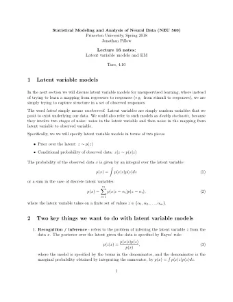
Latent Variable Models with Gaussian Processes Neil D. Lawrence GP - PowerPoint PPT Presentation

Latent Variable Models with Gaussian Processes Neil D. Lawrence GP Master Class 6th February 2017

Outline Motivating Example Linear Dimensionality Reduction Non-linear Dimensionality Reduction

Motivation for Non-Linear Dimensionality Reduction USPS Data Set Handwritten Digit ◮ 3648 Dimensions ◮ 64 rows by 57 columns

Motivation for Non-Linear Dimensionality Reduction USPS Data Set Handwritten Digit ◮ 3648 Dimensions ◮ 64 rows by 57 columns ◮ Space contains more than just this digit.

Motivation for Non-Linear Dimensionality Reduction USPS Data Set Handwritten Digit ◮ 3648 Dimensions ◮ 64 rows by 57 columns ◮ Space contains more than just this digit. ◮ Even if we sample every nanosecond from now until the end of the universe, you won’t see the original six!

Simple Model of Digit Rotate a ’Prototype’

MATLAB Demo demDigitsManifold([1 2], ’all’)

MATLAB Demo demDigitsManifold([1 2], ’all’) 0.1 0.05 PC no 2 0 -0.05 -0.1 -0.1 -0.05 0 0.05 0.1 PC no 1

MATLAB Demo demDigitsManifold([1 2], ’sixnine’ ) 0.1 0.05 PC no 2 0 -0.05 -0.1 -0.1 -0.05 0 0.05 0.1 PC no 1

Low Dimensional Manifolds Pure Rotation is too Simple ◮ In practice the data may undergo several distortions. ◮ e.g. digits undergo ‘thinning’, translation and rotation. ◮ For data with ‘structure’: ◮ we expect fewer distortions than dimensions; ◮ we therefore expect the data to live on a lower dimensional manifold. ◮ Conclusion: deal with high dimensional data by looking for lower dimensional non-linear embedding.

Notation q — dimension of latent / embedded space p — dimension of data space n — number of data points � ⊤ = � � ∈ ℜ n × p data, Y = � y 1 , : , . . . , y n , : y : , 1 , . . . , y : , p � ⊤ = � � centred data, ˆ ∈ ℜ n × p , Y = � ˆ y 1 , : , . . . , ˆ y n , : y : , 1 , . . . , ˆ ˆ y : , p y i , : = y i , : − µ ˆ � ⊤ = � � ∈ ℜ n × q latent variables, X = � x 1 , : , . . . , x n , : x : , 1 , . . . , x : , q mapping matrix, W ∈ ℜ p × q a i , : is a vector from the i th row of a given matrix A a : , j is a vector from the j th row of a given matrix A

Reading Notation X and Y are design matrices Y ⊤ ˆ ◮ Data covariance given by 1 n ˆ Y n cov ( Y ) = 1 i , : = 1 � Y ⊤ ˆ y ⊤ ˆ y i , : ˆ ˆ Y = S . n n i = 1 ◮ Inner product matrix given by YY ⊤ � � k i , j = y ⊤ K = k i , j i , : y j , : i , j ,

Linear Dimensionality Reduction ◮ Find a lower dimensional plane embedded in a higher dimensional space. ◮ The plane is described by the matrix W ∈ ℜ p × q . y = Wx + µ x 2 −→ x 1 y 2 y 3 y 1 Figure: Mapping a two dimensional plane to a higher dimensional space in a linear way. Data are generated by corrupting points on the plane with noise.

Linear Dimensionality Reduction Linear Latent Variable Model ◮ Represent data, Y , with a lower dimensional set of latent variables X . ◮ Assume a linear relationship of the form y i , : = Wx i , : + ǫ i , : , where � � 0 , σ 2 I ǫ i , : ∼ N .

Linear Latent Variable Model Probabilistic PCA ◮ Define linear-Gaussian X relationship between W latent variables and data. σ 2 Y n � � � y i , : | Wx i , : , σ 2 I p ( Y | X , W ) = N i = 1

Linear Latent Variable Model Probabilistic PCA ◮ Define linear-Gaussian X relationship between W latent variables and data. σ 2 ◮ Standard Latent Y variable approach: n � � � y i , : | Wx i , : , σ 2 I p ( Y | X , W ) = N i = 1

Linear Latent Variable Model Probabilistic PCA X W ◮ Define linear-Gaussian relationship between latent variables and σ 2 Y data. ◮ Standard Latent variable approach: n ◮ Define Gaussian prior � � � y i , : | Wx i , : , σ 2 I p ( Y | X , W ) = N over latent space , X . i = 1 n � � � N x i , : | 0 , I p ( X ) = i = 1

Linear Latent Variable Model X W Probabilistic PCA ◮ Define linear-Gaussian relationship between σ 2 Y latent variables and data. ◮ Standard Latent n variable approach: � � � y i , : | Wx i , : , σ 2 I p ( Y | X , W ) = N ◮ Define Gaussian prior i = 1 over latent space , X . n � ◮ Integrate out latent � � p ( X ) = N x i , : | 0 , I variables . i = 1 n � y i , : | 0 , WW ⊤ + σ 2 I � � p ( Y | W ) = N i = 1

Computation of the Marginal Likelihood � � 0 , σ 2 I x i , : ∼ N ( 0 , I ) , ǫ i , : ∼ N y i , : = Wx i , : + ǫ i , : ,

Computation of the Marginal Likelihood � � 0 , σ 2 I x i , : ∼ N ( 0 , I ) , ǫ i , : ∼ N y i , : = Wx i , : + ǫ i , : , Wx i , : ∼ N � 0 , WW ⊤ � ,

Computation of the Marginal Likelihood � � 0 , σ 2 I x i , : ∼ N ( 0 , I ) , ǫ i , : ∼ N y i , : = Wx i , : + ǫ i , : , Wx i , : ∼ N � 0 , WW ⊤ � , 0 , WW ⊤ + σ 2 I � � Wx i , : + ǫ i , : ∼ N

Linear Latent Variable Model II Probabilistic PCA Max. Likelihood Soln (Tipping and Bishop, 1999) W σ 2 Y n � y i , : | 0 , WW ⊤ + σ 2 I � � p ( Y | W ) = N i = 1

Linear Latent Variable Model II Probabilistic PCA Max. Likelihood Soln (Tipping and Bishop, 1999) n N � y i , : | 0 , C � , � C = WW ⊤ + σ 2 I p ( Y | W ) = i = 1

Linear Latent Variable Model II Probabilistic PCA Max. Likelihood Soln (Tipping and Bishop, 1999) n N � y i , : | 0 , C � , � C = WW ⊤ + σ 2 I p ( Y | W ) = i = 1 log p ( Y | W ) = − n 2 log | C | − 1 � � C − 1 Y ⊤ Y 2tr + const. If U q are first q principal eigenvectors of n − 1 Y ⊤ Y and the corresponding eigenvalues are Λ q ,

Linear Latent Variable Model II Probabilistic PCA Max. Likelihood Soln (Tipping and Bishop, 1999) n N � y i , : | 0 , C � , � C = WW ⊤ + σ 2 I p ( Y | W ) = i = 1 log p ( Y | W ) = − n 2 log | C | − 1 � � C − 1 Y ⊤ Y 2tr + const. If U q are first q principal eigenvectors of n − 1 Y ⊤ Y and the corresponding eigenvalues are Λ q , � 1 � W = U q LR ⊤ , Λ q − σ 2 I 2 L = where R is an arbitrary rotation matrix.

Di ffi culty for Probabilistic Approaches ◮ Propagate a probability distribution through a non-linear mapping. ◮ Normalisation of distribution becomes intractable. y j = f j ( x ) x 2 −→ x 1 Figure: A three dimensional manifold formed by mapping from a two dimensional space to a three dimensional space.

Di ffi culty for Probabilistic Approaches y 1 = f 1 ( x ) −→ y 2 x y 2 = f 2 ( x ) y 1 Figure: A string in two dimensions, formed by mapping from one dimension, x , line to a two dimensional space, [ y 1 , y 2 ] using nonlinear functions f 1 ( · ) and f 2 ( · ).

Di ffi culty for Probabilistic Approaches y = f ( x ) + ǫ −→ p ( x ) p ( y ) Figure: A Gaussian distribution propagated through a non-linear � 0 , 0 . 2 2 � mapping. y i = f ( x i ) + ǫ i . ǫ ∼ N and f ( · ) uses RBF basis, 100 centres between -4 and 4 and ℓ = 0 . 1. New distribution over y (right) is multimodal and di ffi cult to normalize.

Linear Latent Variable Model III Dual Probabilistic PCA ◮ Define linear-Gaussian W relationship between X latent variables and data. σ 2 Y n � � y i , : | Wx i , : , σ 2 I � p ( Y | X , W ) = N i = 1

Linear Latent Variable Model III Dual Probabilistic PCA ◮ Define linear-Gaussian W relationship between X latent variables and data. σ 2 ◮ Novel Latent variable Y approach: n � � y i , : | Wx i , : , σ 2 I � p ( Y | X , W ) = N i = 1

Linear Latent Variable Model III Dual Probabilistic PCA W X ◮ Define linear-Gaussian relationship between latent variables and σ 2 Y data. ◮ Novel Latent variable approach: n ◮ Define Gaussian prior � � y i , : | Wx i , : , σ 2 I � p ( Y | X , W ) = N over parameters , W . i = 1 p � � � p ( W ) = N w i , : | 0 , I i = 1

Latent Variable Models with Gaussian Processes Neil D. Lawrence GP - PowerPoint PPT Presentation

Latent Variable Models with Gaussian Processes Neil D. Lawrence GP Master Class 6th February 2017 Outline Motivating Example Linear Dimensionality Reduction Non-linear Dimensionality Reduction Outline Motivating Example Linear

Distributed Variational Inference in Sparse Gaussian Process Regression and Latent Variable Models

1 Latent variable models In the next section we will discuss latent variable models for

Learning Latent Variable Models through Tensor Methods Anima Anandkumar U.C. Irvine Challenges

Latent Variable Models CS3750 Xiaoting Li 1 Out utli line Latent Variable Models

Latent Force Models and Multiple Output Gaussian Processes Neil D. Lawrence work with Magnus

Latent Force Models with Gaussian Processes Neil D. Lawrence Bayesian Research Kitchen,

Learning Overcomplete Latent Variable Models through Tensor Methods Anima Anandkumar UC Irvine

Case Study: Approximate Bayesian Inference for Latent Gaussian Models by Using Integrated Nested

E ffi cient Modeling of Latent Information in Supervised Learning using Gaussian Processes

Outline Latent Variable Generative Models Cooperative Vector Quantizer Model Model

Part III: Latent Tree Models Le Song ICML 2012 Tutorial on Spectral Algorithms for Latent

Piecewise Bounds for Estimating Bernoulli- Logistic Latent Gaussian Models Mohammad Emtiyaz Khan

Learning Overcomplete Latent Variable Models through Tensor Methods Majid Janzamin UC Irvine

Pengtao Xie Joint work with Yuntian Deng and Eric Xing Carnegie Mellon University 1 Latent

Maximum Reconstruction Estimation for Generative Latent-Variable Models Yong Cheng joint work

Guaranteed Learning of Latent Variable Models through Tensor Methods Furong Huang University of

Stochastic (Partial) Differential Equations and Gaussian Processes Simo Srkk Aalto

Latent Variable models for GWAs Oliver Stegle Machine Learning and Computational Biology Research

CSci 8980: Advanced Topics in Graphical Models Gaussian Processes Instructor: Arindam Banerjee

Discriminative Regularization for Latent Variable Models with Applications to Electrocardiography

Latent Variable Models and Expectation Maximization Oliver Schulte - CMPT 726 Bishop PRML Ch. 9

Language and Document Analysis: Motivating Latent variable Models Wray Buntine National ICT

Discrete Latent Variable Models Stefano Ermon, Aditya Grover Stanford University Lecture 15

Empirical Study of the Benefits of Overparameterization in Learning Latent Variable Models