Latent Transition Analysis Exercises We are going to use Mplus to - PDF document

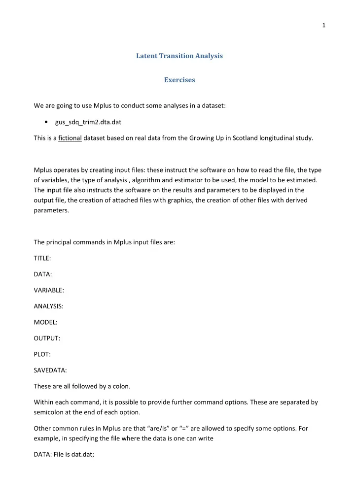
1 Latent Transition Analysis Exercises We are going to use Mplus to conduct some analyses in a dataset: • gus_sdq_trim2.dta.dat This is a fictional dataset based on real data from the Growing Up in Scotland longitudinal study. Mplus operates by creating input files: these instruct the software on how to read the file, the type of variables, the type of analysis , algorithm and estimator to be used, the model to be estimated. The input file also instructs the software on the results and parameters to be displayed in the output file, the creation of attached files with graphics, the creation of other files with derived parameters. The principal commands in Mplus input files are: TITLE: DATA: VARIABLE: ANALYSIS: MODEL: OUTPUT: PLOT: SAVEDATA: These are all followed by a colon. Within each command, it is possible to provide further command options. These are separated by semicolon at the end of each option. Other common rules in Mplus are that “are/is” or “=” are allowed to specify some options. For example, in specifying the file where the data is one can write DATA: File is dat.dat;

2 or DATA: File = dat.dat; Hyphen (-) are used to indicate a list of variables or numbers. Items in a list can be separated by space or commas. Exclamation marks (!) are used to write comments in the input which are not read by the software. What follows the ! in the line is skipped by the software. A SHORT INTRODUCTION TO MPLUS COMMANDS TITLE: allows you to provide a title to the file (text is free). DATA: is used to specify where the data are (the file(s) to be used) and their format and other options (if necessary). It is common to create .dat files (or .txt etc.) that contain data in person-level format (one row for each individual, with values for variables in columns). Do not include variable names in the data file columns. It is possible to specify a path to the data (e.g. C:\my files\datac1.dat). An important option in the DATA: command is LISTWISE= ON , which instructs Mplus to conduct analyses with listwise deletion of cases with one or more missing data in the variables of interest. From version 5 of Mplus the default option is to include cases with missing values on some of the variables in the model. VARIABLE: This command is used to provide names to the variables in the dataset and specify what types of variables they are (their scale) etc. Important options are: NAMES = � list the names of the variables in the dataset. e.g.: NAMES = a b c d male; USEVARIABLE = � list the variables that will be used in the analyses or models. Not necessary if you will be using all the variables in the dataset. Note that if a variable is specified after USEVARIABLE it will be included in the models specified under MODEL: even if not invoked specifically in the MODEL: command. CATEGORICAL, NOMINAL, COUNT = � are used to define a list of dependent variables as ordered categorical (or binary), nominal (unordered), or count variables respectively. Categorical, nominal and count variables that are not treated as dependent should NOT be listed under the CATEGORICAL etc. command. For example, variable “male” should not be listed under CATEGORICAL since it is not going to be used as a dependent variable in the model. e.g. CATEGORICAL = a, b, c, d;

3 MISSING= � specified the value (or a character such as . or *) used to identify a missing value for one or more variables. If all the variables use the same missing value indicator (e.g. -999), write: MISSING = all (-999); IDVARIABLE is used to indicate the identifier for each observation or case in the dataset. This is necessary if you want to create data files after the analyses (SAVEDATA: command) and want to use them for further analyses: in this case, the file saved with SAVEDATA will contain IDs for the observations. e.g.: IDVARIABLE = fullid; CLUSTER is used to indicate a clustering variable (e.g. school, group). This is necessary for multilevel analyses or for analysis that adjust for clustering (option: COMPLEX in ANALYSIS: command) CLASSES is used to specify names of latent categorical variables and the number of classes (between parentheses). If we want to estimate a model with a latent variable called mastery with 2 classes we could write: CLASSES = mastery (2); ANALYSIS: Is used to specify the type of analysis and other options in the analyses (e.g. type of estimator). TYPE of analysis invokes a specific type of analysis among a range of options (e.g. EFA = exploratory factor analysis) TYPE=BASIC invokes descriptive statistics on the variables included by USEVARIABLE. In order to run Latent Class Analysis, Latent Transition Analysis, or other mixture models (GMM or LCGA, etc.) one has to invoke TYPE=MIXTURE; The default estimator for this type of analysis is MLR (maximum likelihood with robust standard errors and chi-square). Once can invoke another estimator by writing the name of the estimator after ESTIMATOR =....; In the ANALYSIS one can also change the number of initial stage starts and final stage optimizations of the EM algorithm by using option STARTS, for example: STARTS = 100 20; It is also possible to change the number of initial stage iterations in the EM algorithm using option STITERATIONS, for example specifying: STITERATIONS = 20; PROCESSORS can also be used to devote more computer memory resources (processors) to the estimation process (default is PROCESSORS = 1). MODEL: The model command allows to specify a model, constrain parameters, test parameter constraints. ON is short for “regressed on” and defines regression relationships e.g.: y on x; y on male; y on x male;

4 Variables within brackets refer to the variable means (if interval variables) or to variable thresholds in the case of categorical variables. The different thresholds of a categorical variable are labelled using $ followed by the threshold number. If variable a has three response categories, it will have 2 thresholds indicated by: [a$1]; [a$2]; The star sign * is used to free a parameter, if followed by a number it uses a user-specified starting value. For example, to provide starting value of -1 for first threshold of a, one would write: [a$1*-1]; The at sign @ fixes a parameter at a user-specified value. For example, to fix the second threshold of a to -2, one would write: [a$2@-2]; Parentheses are used to name or to constrain a parameter. Names are provided when letters are within parentheses. E.g. to name the thresholds of variable “a” p1 and p2: [a$1] (p1); [a$2] (p2); These parameters can then be constrained using the MODEL CONSTRAINT: option in the MODEL command. For example, to impose equality constraints on these two thresholds for variable “a”: MODEL CONSTRAINT: p1 = p2; The same equality constraint can be imposed using numbers between parentheses: if thresholds of variables a and b are constrained equal, write: [a$1] (1); [b$1] (1); OUTPUT: Specifies the information to be reported in the output file. SAVEDATA: Instructs the programme to create a file with parameters estimated. FILE is used to give a name to new file. For example: FILE IS analsis1.dat; SAVE is uses to specify what information can be saved in the file. CPROB will save posterior latent class probabilities and modal class assignment for each individual included in the analyses. If an IDVARIABLE is specified in VARIABLE command, the file will contain ID variable information, and it will be possible to match-merge the file with other files for further analyses. E.g.: FILE is analysis1.dat; SAVE = CPROB;