Latent Semantic Analysis (Tutorial) Alex Thomo 1 Eigenvalues and - PDF document

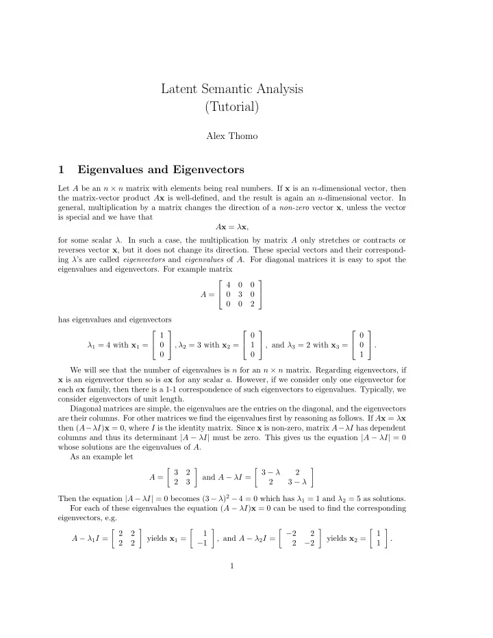
Latent Semantic Analysis (Tutorial) Alex Thomo 1 Eigenvalues and Eigenvectors Let A be an n × n matrix with elements being real numbers. If x is an n -dimensional vector, then the matrix-vector product A x is well-defined, and the result is again an n -dimensional vector. In general, multiplication by a matrix changes the direction of a non-zero vector x , unless the vector is special and we have that A x = λ x , for some scalar λ . In such a case, the multiplication by matrix A only stretches or contracts or reverses vector x , but it does not change its direction. These special vectors and their correspond- ing λ ’s are called eigenvectors and eigenvalues of A . For diagonal matrices it is easy to spot the eigenvalues and eigenvectors. For example matrix ⎡ ⎤ 4 0 0 A = 0 3 0 ⎣ ⎦ 0 0 2 has eigenvalues and eigenvectors ⎡ ⎤ ⎡ ⎤ ⎡ ⎤ 1 0 0 ⎦ , λ 2 = 3 with x 2 = ⎦ , and λ 3 = 2 with x 3 = ⎦ . λ 1 = 4 with x 1 = 0 1 0 ⎣ ⎣ ⎣ 0 0 1 We will see that the number of eigenvalues is n for an n × n matrix. Regarding eigenvectors, if x is an eigenvector then so is a x for any scalar a . However, if we consider only one eigenvector for each a x family, then there is a 1-1 correspondence of such eigenvectors to eigenvalues. Typically, we consider eigenvectors of unit length. Diagonal matrices are simple, the eigenvalues are the entries on the diagonal, and the eigenvectors are their columns. For other matrices we find the eigenvalues first by reasoning as follows. If A x = λ x then ( A − λ I ) x = 0, where I is the identity matrix. Since x is non-zero, matrix A − λ I has dependent columns and thus its determinant | A − λ I | must be zero. This gives us the equation | A − λ I | = 0 whose solutions are the eigenvalues of A . As an example let � � � � 3 2 3 − λ 2 A = and A − λ I = 2 3 2 3 − λ Then the equation | A − λ I | = 0 becomes (3 − λ ) 2 − 4 = 0 which has λ 1 = 1 and λ 2 = 5 as solutions. For each of these eigenvalues the equation ( A − λ I ) x = 0 can be used to find the corresponding eigenvectors, e.g. � 2 � 1 � − 2 � � � � � 2 1 2 A − λ 1 I = yields x 1 = , and A − λ 2 I = yields x 2 = . 2 2 − 1 2 − 2 1 1

In general, for an n × n matrix A , the determinant | A − λ I | will give a polynomial of degree n which has n roots. In other words, the equation | A − λ I | = 0 will give n eigenvalues. Let us create a matrix S with columns the n eigenvectors of A . We have that AS = A [ x 1 , . . . , x n ] = A x 1 + . . . + A x n = λ 1 x 1 + . . . + λ n x n ⎡ ⎤ λ 1 ... = [ x 1 , . . . , x n ] ⎦ . ⎢ ⎥ ⎣ λ n = S Λ , where Λ is the above diagonal matrix with the eigenvalues of A along its diagonal. Now suppose that the above n eigenvectors are linearly independent. This is true when the matrix has n distinct eigenvalues. Then matrix S is invertible and by mutiplying both sides of AS = S Λ we have A = S Λ S − 1 . So, we were able to “diagonalize” matrix A in terms of the diagonal matrix Λ spelling the eigenvalues of A along its diagonal. This was possible because matrix S was invertible. When there are fewer than n eigenvalues then it might happen that the diagonalization is not possible. In such a case the matrix is “defective” having too few eigenvectors. In this tutorial, for reasons to be clear soon we will be interested in symmetric matrices ( A = A T ). For n × n symmetric matrices it has been shown that that they always have real eigenvalues and their eigenvectors are perpendicular. As such we have that ⎡ x T ⎤ ⎡ ⎤ 1 1 . S T S = ... . ⎦ [ x 1 , . . . , x n ] = ⎦ = I. ⎢ ⎥ ⎢ ⎥ . ⎣ ⎣ x T 1 n In other words, for symmetric matrices, S − 1 is S T (which can be easily obtained) and we have A = S Λ S T . 2

2 Singular Value Decomposition Now let A be an m × n matrix with entries being real numbers and m > n . Let us consider the n × n square matrix B = A T A . It is easy to verify that B is symmetric; namely B T = ( A T A ) T = A T ( A T ) T = A T A = B ). It has been shown that the eigenvalues of such matrices ( A T A ) are real non-negative numbers. Since they are non-negative we can write them in decreasing order as squares of non-negative real numbers: σ 2 1 ≥ . . . ≥ σ 2 n . For some index r (possibly n ) the first r numbers σ 1 , . . . , σ r are positive whereas the rest are zero. For the above eigenvalues, we know that the corresponding eigenvectors x 1 , . . . , x r are perpendicular. Furthemore, we normalize them to have length 1. Let S 1 = [ x 1 , . . . , x r ] . 1 1 We create now the vectors y 1 = σ 1 A x 1 , . . . , y r = σ r A x r . These are perpendicular m -dimensional vectors of length 1 (orthonormal vectors) because � 1 � T 1 y T = A x i A x j i y j σ 1 σ j 1 i A T A x j x T = σ i σ j 1 x T = i B x j σ i σ j 1 x T i σ 2 = j x j σ i σ j σ j x T = i x j σ i is 0 for i ̸ = j and 1 for i = j (since x T i x j = 0 for i ̸ = j and x T i x i = 1). Let S 2 = [ y 1 , . . . , y r ] . We have y T j A x i = y T j ( σ i y i ) = σ i y T j y i , which is 0 if i ̸ = j , and σ i if i = j . From this we have S T 2 AS 1 = Σ , where Σ is the diagonal r × r matrix with σ 1 , . . . , σ r along the diagonal. Observe that S T 2 is r × m , A is m × n , and S 1 is n × r , and thus the above matrix multiplication is well defined. Since S 2 and S 1 have orthonormal columns, S 2 S T 2 = I m × m and S 1 S T 1 = I n × n , where I m × m and I n × n are the m × m and n × n identity matrices. Thus, by multiplying the above equality by S 2 on the left and S 1 on the right, we have A = S 2 Σ S T 1 . Reiterating, matrix Σ is diagonal and the values along the diagonal are σ 1 , . . . , σ r , which are called singular values . They are the square roots of the eigenvalues of A T A and thus completely determined by A . The above decomposition of A into S T 2 AS 1 is called singular value decomposition . For the ease of notation, let us denote S 2 by S and S 1 by U (getting thus rid of the subscripts). Then A = S Σ U T . 3

3 Latent Semantic Indexing Latent Semantic Indexing (LSI) is a method for discovering hidden concepts in document data. Each document and term (word) is then expressed as a vector with elements corresponding to these concepts. Each element in a vector gives the degree of participation of the document or term in the corresponding concept. The goal is not to describe the concepts verbally, but to be able to represent the documents and terms in a unified way for exposing document-document, document-term, and term-term similarities or semantic relationship which are otherwise hidden. 3.1 An Example Suppose we have the following set of five documents d 1 : Romeo and Juliet. d 2 : Juliet: O happy dagger! d 3 : Romeo died by dagger. d 4 : “Live free or die”, that’s the New-Hampshire’s motto. d 5 : Did you know, New-Hampshire is in New-England. and a search query: dies, dagger . Clearly, d 3 should be ranked top of the list since it contains both dies, dagger . Then, d 2 and d 4 should follow, each containing a word of the query. However, what about d 1 and d 5 ? Should they be returned as possibly interesting results to this query? As humans we know that d 1 is quite related to the query. On the other hand, d 5 is not so much related to the query. Thus, we would like d 1 but not d 5 , or di ff erently said, we want d 1 to be ranked higher than d 5 . The question is: Can the machine deduce this? The answer is yes, LSI does exactly that. In this example, LSI will be able to see that term dagger is related to d 1 because it occurs together with the d 1 ’s terms Romeo and Juliet , in d 2 and d 3 , respectively. Also, term dies is related to d 1 and d 5 because it occurs together with the d 1 ’s term Romeo and d 5 ’s term New-Hampshire in d 3 and d 4 , respectively. LSI will also weigh properly the discovered connections; d 1 more is related to the query than d 5 since d 1 is “doubly” connected to dagger through Romeo and Juliet , and also connected to die through Romeo , whereas d 5 has only a single connection to the query through New-Hampshire . 3.2 SVD for LSI Formally let A be the m × n term-document matrix of a collection of documents. Each column of A corresponds to a document. If term i occurs a times in document j then A [ i, j ] = a . The dimensions of A , m and n , correspond to the number of words and documents, respectively, in the collection. For our example, matrix A is: d 1 d 2 d 3 d 4 d 5 romeo 1 0 1 0 0 juliet 1 1 0 0 0 happy 0 1 0 0 0 dagger 0 1 1 0 0 live 0 0 0 1 0 die 0 0 1 1 0 free 0 0 0 1 0 new-hampshire 0 0 0 1 1 4