Lab 5: 16 th April 2012 Exercises on Neural Networks 1. What are the - PDF document

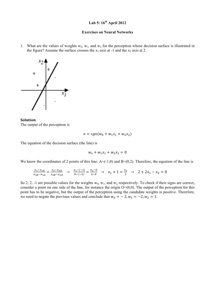
Lab 5: 16 th April 2012 Exercises on Neural Networks 1. What are the values of weights w 0 , w 1 , and w 2 for the perceptron whose decision surface is illustrated in the figure? Assume the surface crosses the x 1 axis at -1 and the x 2 axis at 2. Solution ¡ The output of the perceptron is ! = !"# ( ! ! + ! ! ! ! + ! ! ! ! ) The equation of the decision surface (the line) is ! ! + ! ! ! ! + ! ! ! ! = 0 We know the coordinates of 2 points of this line: A=(-1,0) and B=(0,2). Therefore, the equation of the line is ! ! ! ! ! ! ! ! ! ! ! ! ! ! ! ( ! ! ) ! ! ! ! ! ! ! ! ! ! ! ! ! = ! ! ! ! ! ! ! ¡ ¡ ¡ → ¡ ¡ ¡ ! ! ( ! ! ) = ! ! ! ¡ ¡ ¡ → ¡ ¡ ¡ ! ! + 1 = ! ¡ ¡ ¡ → ¡ ¡ ¡ 2 + 2 ! ! − ! ! = 0 So 2, 2, -1 are possible values for the weights w 0 , w 1 , and w 2, respectively. To check if their signs are correct, consider a point on one side of the line, for instance the origin O=(0,0). The output of the perceptron for this point has to be negative, but the output of the perceptron using the candidate weights is positive. Therefore, we need to negate the previous values and conclude that ! ! = − ¡ 2 , ! ! = − 2 , ! ! = 1 .

2. (a) Design a two-input perceptron that implements the Boolean function A ∧ ¬ B. (b) Design the two-layer network of perceptrons that implements A XOR B. Solution ¡ (a) The requested perceptron has 3 inputs: A, B, and the constant 1. The values of A and B are 1 (true) or -1 (false). The following table describes the output O of the perceptron: A B O = A ∧ ¬ B -1 -1 -1 -1 1 -1 1 -1 1 1 1 -1 One of the correct decision surfaces (any line that separates the positive point from the negative points would be fine) is shown in the following picture. The line crosses the A axis at 1 and the B axis -1. The equation of the line is ! ! ! ! ! ( ! ! ) ¡ ¡ ¡ ¡ ¡ ¡ ¡ ! ! ! = ! ! ( ! ! ) ¡ ¡ ¡ → ¡ ! = ¡ ! + 1 ¡ ¡ → ¡ ¡ ¡ 1 − ! + ! = 0 So 1, -1, 1 are possible values for the weights w 0 , w 1 , and w 2, respectively. Using this values the output of the perceptron for A=1, B=-1 is negative. Therefore, we need to negate the weights and therefore we can conclude that ! ! = − 1 , ! ! = 1 , ! ! = − 1 . ¡ Solution ¡ (b) A XOR B cannot be calculated by a single perceptron, so we need to build a two-layer network of perceptrons. The structure of the network can be derived by: • Expressing A XOR B in terms of other logical connectives: A XOR B = (A ∧ ¬ B) ∨ ( ¬ A ∧ B) • Defining the perceptrons P 1 and P 2 for (A ∧ ¬ B) and ( ¬ A ∧ B) • Composing the outputs of P 1 and P 2 into a perceptron P 3 that implements o(P 1 ) ∨ o(P 2 ) Perceptron P 1 has been defined above. P 2 can be defined similarly. P 3 is defined in the course slides 1 . In the end, the requested network is the following: NB. The number close to each unit is the weight w 0 . 1 It is defined for 0/1 input values, but it can be easily modified for -1/+1 input values.

3. Consider two perceptrons A and B defined by the threshold expression w 0 +w 1 x 1 +w 2 x 2 >0. Perceptron A has weight values w 0 =1, w 1 =2, w 2 =1 and perceptron B has weight values w 0 =0, w 1 =2, w 2 =1. Is perceptron A more_general_than perceptron B? A is more_general_than B if and only if ∀ instance <x 1 ,x 2 >, B(<x 1 ,x 2 >)=1 à A(<x 1 ,x 2 >)=1. Solution B(<x 1 ,x 2 >) = 1 à 2x 1 +x 2 > 0 à 1+2x 1 +x 2 > 0 à A(<x 1 ,x 2 >) = 1

4. Derive a gradient descent training rule for a single unit with output o , where 2 +…+w n x n +w n x n 2 o=w 0 +w 1 x 1 +w 1 x 1 Solution The gradient descent training rule specifies how the weights are to be changed at each step of the learning procedure so that the prediction error of the unit decreases the most. The derivation of the rule for a linear unit is presented on pages 91-92 of the Mitchell, and on pages 4-6 of the course slides ( ml_2012_lecture_07 ). We can adapt that derivation and consider the output o . ! E ! ( ) = $ ( 2 + … +w n x n x +w n x n x 2 ) $ ( 2 ) ( ) ( ) out x " o x out x " w 0 +w 1 x 1 x +w 1 x 1 x out x " o x " x i x " x i x = ! w i ! w i x # X x # X Therefore, the gradient descent training rule is ! E ! ( ) = ( ) ( ) $ 2 + … +w n x n x +w n x n x 2 $ 2 ( out x " o x ) out x " w 0 +w 1 x 1 x +w 1 x 1 x ( out x " o x ) " x i x " x i x = ! w i ! w i x # X x # X

5. Consider a two-layer feed-forward neural network that has the topology shown in the figure. • X 1 and X 2 are the two inputs. • Z 1 and Z 2 are the two hidden neurons. • Y is the (single) output neuron. • w i , i=1..4, are the weights of the connections from the inputs to the hidden neurons. • w j , j=5..6, are the weights of the connections from the hidden neurons to the output neuron. X 1 X 2 w 3 w 2 w 1 w 4 Z 1 Z 2 w 5 w 6 Y Explain the three phases (i.e., input signal forward, error signal backward, and weight update) of the first training iteration of the Backpropagation algorithm for the current network, given the training example: ( X 1 =x 1 , X 2 =x 2 , Y =y). Please use the following notations for the explanation. • Net 1 , Net 2 , and Net 3 are the net inputs to the Z 1 , Z 2 , and Y neurons, respectively. • o 1 , o 2 , and o 3 are the output values for the Z 1 , Z 2 , and Y neurons, respectively. • f is the activation function used for every neuron in the network, i.e., o k =f(Net k ), k=1..3. E( w ) = (y - o 3 ) 2 / 2 is the error function, where y is the desired network output. • • η is the learning rate • δ 1 , δ 2 , and δ 3 are the error signals for the Z 1 , Z 2 , and Y neurons, respectively. Solution ¡ Propagate the input forward through the network 1. Input the instance (x 1 ,x 2 ) to the network and compute the network outputs o 3 • Net 1 = w 1 x 1 + w 2 x 2 à o 1 =f(Net 1 ) • Net 2 = w 3 x 1 + w 4 x 2 à o 2 =f(Net 2 ) • Net 3 = w 5 f(Net 1 )+w 6 f(Net 2 ) à o 3 =f(w 5 f(Net 1 )+w 6 f(Net 2 )) Propagate the error backward through the network E( w ) = (y - o 3 ) 2 / 2 = (y-f(w 5 f(Net 1 )+w 6 f(Net 2 ))) 2 • 2. Calculate the error term of out unit Y • δ 3 =f’(f(w 5 f(Net 1 )+w 6 f(Net 2 )))*(y-f(w 5 f(Net 1 )+w 6 f(Net 2 ))) 3. Calculate the error of the 2 hidden units • δ 2 =f’(f(Net 2 ) δ 3 δ 1 =f’(f(Net 1 ) δ 3 4. Update the network weights • w 1 ß w 1 + η δ 1 w 1 • w 2 ß w 2 + η δ 2 w 2 • w 3 ß w 3 + η δ 1 w 3 • w 4 ß w 4 + η δ 2 w 4 • w 5 ß w 5 + η δ 3 w 5 • w 6 ß w 6 + η δ 3 w 6

6. In the Back-Propagation learning algorithm, what is the object of the learning? Does the Back- Propagation learning algorithm guarantee to find the global optimum solution? Solution ¡ The ¡object ¡is ¡to ¡learn ¡the ¡weights ¡of ¡the ¡interconnections ¡between ¡the ¡inputs ¡and ¡the ¡hidden ¡units ¡and ¡ between ¡the ¡hidden ¡units ¡and ¡the ¡output ¡units. ¡The ¡algorithms ¡attempts ¡to ¡minimize ¡the ¡squared ¡error ¡ between ¡the ¡network ¡output ¡values ¡and ¡the ¡target ¡values ¡of ¡these ¡outputs. ¡ The ¡ learning algorithm does not guarantee to find the global optimum solution. It guarantees to find at least a local minimum of the error function.