L2AP: Fast Cosine Similarity Search With Prefix L-2 Norm Bounds - PowerPoint PPT Presentation
L2AP: Fast Cosine Similarity Search With Prefix L-2 Norm Bounds David C. Anastasiu and George Karypis University of Minnesota, Minneapolis, MN, USA April 3, 2014 1 / 27 All-Pairs Similarity Search (APSS) Goal For each object in a set,
L2AP: Fast Cosine Similarity Search With Prefix L-2 Norm Bounds David C. Anastasiu and George Karypis University of Minnesota, Minneapolis, MN, USA April 3, 2014 1 / 27
All-Pairs Similarity Search (APSS) Goal ◮ For each object in a set, find all other set objects with a similarity value of at least t (its neighbors) Applications ◮ Near-duplicate Document Detection ◮ Clustering ◮ Query Refinement ◮ Collaborative Filtering ◮ Semi-supervised Learning ◮ Information Retrieval 2 / 27
Outline 1. Problem Description 2. Solution framework 3. Index construction 4. Candidate generation 5. Candidate verification 6. Experimental Evaluation 6.1 Efficiency testing 6.2 Effectiveness testing 7. Conclusion 3 / 27
Problem Description ◮ D , sparse matrix of size n × m ◮ x , row vector for row x in D ◮ rows unit-length normalized, x x = || x || ⇒ || x || = 1 xy T ◮ sim ( x , y ) = cos ( x , y ) = || x ||×|| y || = xy T = � m j = 1 x j × y j 4 / 27
Problem Description ◮ Na¨ ıve solution: compute similarity of each object with all others, keep results ≥ t . ◮ Equivalent to sparse matrix-matrix multiplication, followed by a filter operation: APSS ∼ DD T . ≥ t for each row x = 1 , . . . , n do for each row y = 1 , . . . , n do if x � = y & sim ( x , y ) > t then Add { x , y , sim ( x , y ) } to result × = DD T D T D 5 / 27
Problem Description ◮ Main idea : Use the similarity threshold t and theoretical bounds to prune the search space a = � 0.12, , 0.37, 0.22, , 0.47, 0.75, 0.13 � b = � � , 0.50, 0.65, , 0.05, 0.35, 0.45, c = � 0.96, 0.28, 0.01, , , , , � A [ b ] = 0 . 0000 A [ c ] = 0 . 0000 t = 0 . 5 6 / 27
Problem Description ◮ Main idea : Use the similarity threshold t and theoretical bounds to prune the search space a = � 0.12, , 0.37, 0.22, , 0.47, 0.75, 0.13 � b = � � , 0.50, 0.65, , 0.05, 0.35, 0.45, c = � 0.96, 0.28, 0.01, , , , , � A [ b ] = 0 . 0000 A [ c ] = 0 . 1152 t = 0 . 5 6 / 27
Problem Description ◮ Main idea : Use the similarity threshold t and theoretical bounds to prune the search space a = � 0.12, , 0.37, 0.22, , 0.47, 0.75, 0.13 � b = � � , 0.50, 0.65, , 0.05, 0.35, 0.45, c = � 0.96, 0.28, 0.01, , , , , � A [ b ] = 0 . 0000 A [ c ] = 0 . 1152 t = 0 . 5 6 / 27
Problem Description ◮ Main idea : Use the similarity threshold t and theoretical bounds to prune the search space a = � 0.12, , 0.37, 0.22, , 0.47, 0.75, 0.13 � b = � � , 0.50, 0.65, , 0.05, 0.35, 0.45, c = � 0.96, 0.28, 0.01, , , , , � A [ b ] = 0 . 2405 A [ c ] = 0 . 1189 t = 0 . 5 6 / 27
Problem Description ◮ Main idea : Use the similarity threshold t and theoretical bounds to prune the search space a = � 0.12, , 0.37, 0.22, , 0.47, 0.75, 0.13 � b = � � , 0.50, 0.65, , 0.05, 0.35, 0.45, c = � 0.96, 0.28, 0.01, , , , , � A [ b ] = 0 . 2405 A [ c ] = 0 . 1189 t = 0 . 5 6 / 27
Problem Description ◮ Main idea : Use the similarity threshold t and theoretical bounds to prune the search space a = � 0.12, , 0.37, 0.22, , 0.47, 0.75, 0.13 � b = � � , 0.50, 0.65, , 0.05, 0.35, 0.45, c = � 0.96, 0.28, 0.01, , , , , � A [ b ] = 0 . 2405 A [ c ] = 0 . 1189 t = 0 . 5 6 / 27
Problem Description ◮ Main idea : Use the similarity threshold t and theoretical bounds to prune the search space a = � 0.12, , 0.37, 0.22, , 0.47, 0.75, 0.13 � b = � � , 0.50, 0.65, , 0.05, 0.35, 0.45, c = � 0.96, 0.28, 0.01, , , , , � A [ b ] = 0 . 4050 A [ c ] = 0 . 1189 t = 0 . 5 6 / 27
Problem Description ◮ Main idea : Use the similarity threshold t and theoretical bounds to prune the search space a = � 0.12, , 0.37, 0.22, , 0.47, 0.75, 0.13 � b = � � , 0.50, 0.65, , 0.05, 0.35, 0.45, c = � 0.96, 0.28, 0.01, , , , , � A [ b ] = 0 . 7425 A [ c ] = 0 . 1189 t = 0 . 5 6 / 27
Problem Description ◮ Main idea : Use the similarity threshold t and theoretical bounds to prune the search space a = � 0.12, , 0.37, 0.22, , 0.47, 0.75, 0.13 � b = � � , 0.50, 0.65, , 0.05, 0.35, 0.45, c = � 0.96, 0.28, 0.01, , , , , � A [ b ] = 0 . 7425 A [ c ] = 0 . 1189 t = 0 . 5 6 / 27
Extensions to the na¨ ıve approach ◮ Leverage sparsity in D . Build an inverted index . ◮ Leverage commutativity of cos ( x , y ) . (Sarawagi and Kirpal, 2004) . ◮ Build a partial index . (Chaudhuri et al., 2006) 7 / 27
AllPairs Framework AllPairs : for each row x = 1 , . . . , n do Find similarity candidates for x using current inverted index (candidate generation) Complete similarity computation and prune unpromising candidates (candidate verification) Index enough of x to ensure all valid similar- ity pairs are discovered (index construction) 8 / 27
What we index ◮ We index x ′′ , the suffix of x . x ′′ p = � 0 , . . . , 0 , x p , . . . , x m � is the suffix of x starting at feature p . ◮ x ′ is the un-indexed prefix of x . x ′ p = � x 1 , . . . , x p − 1 , 0 , . . . , 0 � is x ’s prefix ending at p − 1. a = � 0.12, , 0.47, 0.75, 0.13 � , 0.37, 0.22, a ′′ 4 = � , 0.47, 0.75, 0.13 � , , , 0.22, a ′ 4 = � 0.12, � , 0.37, , , , , ◮ x = x ′ + x ′′ � p − 1 � m xy T = j = 1 x j × y j + j = p x j × y j ◮ x ′ p y T x ′′ p y T = + ◮ cos ( x , y ) ≤ || x || × || y || (Cauchy–Schwarz inequality) 9 / 27
Index Construction ◮ Add a minimum number of non-zero features j of x to the inverted index lists I j (index filtering). for each column j = 1 , . . . , m s.t. x j > 0 do if sim ( x ′ j + 1 , y ) ≥ t , ∀ y > x then I j ← I j ∪ { ( x , x j ) } 10 / 27
Index Construction ◮ By the Cauchy–Schwarz inequality , cos ( x ′ j , y ) ≤ || x ′ j || × || y || = || x ′ j || , since || y || = 1 (bound b 3 ). ◮ We store || x ′ j || along with x j in the index to use for later pruning. a = � 0.12, , 0.47, 0.75, 0.13 � , 0.37, 0.22, || a j || = � 0.12, 0.12, 0.39, 0.45, 0.45, 0.65, 0.99, 1.00 � 11 / 27
Index Construction ◮ Let w = � max z 1 , . . . , max z m � , the vector of max column z z values in D . We can estimate sim ( x ′ j , y ) ≤ sim ( x ′ j , w ) . ◮ Leverage an order of D ’s rows. Order rows in decreasing max row value ( || z || ∞ ) order. Let w = � min ( x 1 , max ˆ z 1 ) , . . . , min ( x n , max z m ) � . z z Then sim ( x ′ j , y ) ≤ sim ( x ′ j , ˆ w ) , since the y ’s we seek follow x in the row order (bound b 1 , Bayardo et al., 2007). ◮ We use the minimum of the two bounds, min ( b 1 , b 3 ) . ◮ We store ps [ x ] ← min ( sim ( x ′ j , ˆ w ) , || x j || ) to use in later pruning. 12 / 27
Candidate generation ◮ Traverse the inverted index lists I j corresponding to non-zero features j of x and keep track of a partial dot product ( A [ y ] ) for the candidates encountered. for each column j = m , . . . , 1 s.t. x j > 0 do for each ( y , y j ) ∈ I j do if A [ y ] > 0 or sim ( x ′ j , y ) ≥ t then A [ y ] ← A [ y ] + x j × y j A [ y ] ← 0 if A [ y ] + sim ( x ′ j , y ′ j ) < t ◮ Note that we are accumulating the suffix dot product , sim ( x ′′ , y ) . 13 / 27
Candidate generation ◮ Leverage t to prune potential candidates (residual filtering). for each column j = m , . . . , 1 s.t. x j > 0 do for each ( y , y j ) ∈ I j do if A [ y ] > 0 or sim ( x ′ j , y ) ≥ t then A [ y ] ← A [ y ] + x j × y j A [ y ] ← 0 if A [ y ] + sim ( x ′ j , y ′ j ) < t ◮ Accumulate only if A [ y ] > 0 or || x ′ j || ≥ t , since cos ( x ′ j , y ) ≤ || x ′ j || (bound rs 4 ). ◮ Once the ℓ 2 norm of x ′ j falls below t , we ignore potential candidates y if A [ y ] = 0. 14 / 27
Candidate generation ◮ Given w defined as before, sim ( x ′ , y ) ≤ sim ( x ′ , w ) (bound rs 1 , Bayardo et al., 2007). We pre-compute rs 1 = xw T , and roll back the computation as we process each inverted index column j . We stop accumulating new candidates once rs 1 < t . ◮ Candidates can only be those vectors with lower ids. We can improve rs 1 by using max column values of processed columns instead, � w = � max z < x z 1 , . . . , max z < x z m � , thus sim ( x ′ , y ) ≤ sim ( x ′ , � w ) (bound rs 3 ). ◮ We use the best of both bounds, min ( rs 3 , rs 4 ) , during residual filtering. 15 / 27
Candidate generation ◮ Leverage t at common features to prune actual candidates (positional filtering). for each column j = m , . . . , 1 s.t. x j > 0 do for each ( y , y j ) ∈ I j do if A [ y ] > 0 or sim ( x ′ j , y ) ≥ t then A [ y ] ← A [ y ] + x j × y j A [ y ] ← 0 if A [ y ] + sim ( x ′ j , y ′ j ) < t ◮ We estimate sim ( x ′ j , y ′ j ) ≤ || x ′ j || × || y ′ j || ( || y ′ j || is stored in the index), to prune some of the candidates (bound l 2 cg ). ◮ We store || x ′ j || for forward index features to use in future pruning. 16 / 27
Candidate verification ◮ We use the forward index to finish computing the dot products for the encountered candidates, vectors y with A [ y ] > 0. for each y s.t. A [ y ] > 0 do next y if A [ y ] + sim ( x , y ′ ) < t for each column j s.t. y j > 0 ∧ y j / ∈ I j ∧ x j > 0 do A [ y ] ← A [ y ] + x j × y j next y if A [ y ] + sim ( x ′ j , y ′ j ) < t Add { x , y , A [ y ] } to result if A [ y ] > t 17 / 27
Recommend
More recommend
Explore More Topics
Stay informed with curated content and fresh updates.


