K ( t ) = Gy ( t ) y T ( t ) ( K ( t )) u ( t ) = K ( t ) y ( t - PDF document
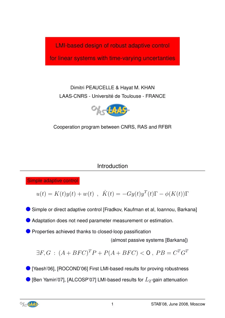
LMI-based design of robust adaptive control for linear systems with time-varying uncertanties Dimitri PEAUCELLE & Hayat M. KHAN LAAS-CNRS - Universit e de Toulouse - FRANCE Cooperation program between CNRS, RAS and RFBR Introduction
LMI-based design of robust adaptive control for linear systems with time-varying uncertanties Dimitri PEAUCELLE & Hayat M. KHAN LAAS-CNRS - Universit´ e de Toulouse - FRANCE Cooperation program between CNRS, RAS and RFBR Introduction Simple adaptive control ˙ K ( t ) = − Gy ( t ) y T ( t ) Γ − φ ( K ( t )) Γ u ( t ) = K ( t ) y ( t ) + w ( t ) , ● Simple or direct adaptive control [Fradkov, Kaufman et al, Ioannou, Barkana] ● Adaptation does not need parameter measurement or estimation. ● Properties achieved thanks to closed-loop passification (almost passive systems [Barkana]) ∃ F, G : ( A + BFC ) T P + P ( A + BFC ) < O , PB = C T G T ● [Yaesh’06], [ROCOND’06] First LMI-based results for proving robustness ● [Ben Yamin’07], [ALCOSP’07] LMI-based results for L 2 -gain attenuation 1 STAB’08, June 2008, Moscow
Introduction Simple adaptive control ˙ K ( t ) = − Gy ( t ) y T ( t ) Γ − φ ( K ( t )) Γ u ( t ) = K ( t ) y ( t ) + w ( t ) , ● SAC is claimed to be robust and to adapt to parametric variations. ● This work is devoted to: ▲ For a class of uncertain systems, provide robust stability conditions. ▲ Conditions are inspired of Robust Control results for uncertain linear systems. ▲ They are in LMI form, therefore numerically testable. ● Outline: ❶ Problem statement : Properties of SAC and definition of uncertain systems ❷ Main result : LMI formulas for proving existence of an attraction domain ❸ Additional result : LMI formulas for estimating the attraction domain ❹ Some clues about the proofs 2 STAB’08, June 2008, Moscow ❶ Problem statement Simple adaptive control ˙ K ( t ) = − Gy ( t ) y T ( t ) Γ − φ ( K ( t )) Γ u ( t ) = K ( t ) y ( t ) + w ( t ) , ● If Γ = O : SAC reduces to SOF ( K ( t ) = K (0) = F ). Stability depends of the choice of F . ● For Γ > O and appropriate choices of G and φ : SAC may be stabilizing whatever initial conditions K (0) . If K ( t ) converges to a fixed point, then K ( ∞ ) = F is stablizing SOF . ● For this presentation: G is assumed given and φ is dead-zone type, defined by φ ( K ) = ψ ( Tr ( K T K )) K where ψ ( k ) = 0 ∀ 0 ≤ k < α ψ ( k ) = k − α ∀ α ≤ k < β β − k 3 STAB’08, June 2008, Moscow
❶ Problem statement Simple adaptive control ˙ K ( t ) = − Gy ( t ) y T ( t ) Γ − φ ( K ( t )) Γ u ( t ) = K ( t ) y ( t ) + w ( t ) , ● φ is dead-zone type, defined by φ ( K ) = ψ ( Tr ( K T K )) K where ψ ( k ) = 0 ∀ 0 ≤ k < α ψ ( k ) = k − α ∀ α ≤ k < β β − k ● The term − Gyy T Γ has properties for ”driving” K to stabilizing values. ● The term − φ ( K ) Γ prevents K to grow too large (Tr ( K T K ) < β ). ● α should be large to keep the adaptation free. ● α and β are assumed given accordingly to implementation constraints. 4 STAB’08, June 2008, Moscow ❶ Problem statement Linear system with affine time-varying uncertainties A ( δ ) B ( δ ) C ( δ ) � �� � � �� � � �� � � � � � � � ¯ ¯ ¯ p p p � � � x = ˙ A 0 + δ p A p x + B 0 + δ p B p u , y = C 0 + δ p C p x . p =1 p =1 p =1 ● Bounded uncertainties δ p ≤ δ p ( t ) ≤ δ p , ● with bounded time derivatives ϑ p ≤ ˙ δ p ( t ) ≤ ϑ p . ● ∆ is the set of all uncertainties, ● ¯ p vertices δ p ∈ { δ p , δ p } , ϑ p ∈ { ϑ p , ϑ p } . ∆ the set of 2 2¯ ▲ Can model some non-linear systems with parametric uncertainties. ▲ Nominal system ( δ = 0 ) assumed to have SOF passifiability property: ∃ F 0 , ∃ D : ˙ x = ( A 0 + B 0 F 0 C 0 ) x + B 0 w , z = GC 0 x + Dw is passive 5 STAB’08, June 2008, Moscow
❷ Main result THM 1 Existence of an attraction domain ● For a chosen scalar ǫ > 0 solve the LMI problem L 1 ( H 1 , H 2 , P p =0 ... ¯ p ) < O p , F p =0 ... ¯ p , D p =0 ... ¯ p , R p =0 ... ¯ p , T p =0 ... ¯ ● If feasible, the solution is such that ▲ F ( δ ) = F 0 + � ¯ p p =1 δ p F p is a robustly stabilizing parameter-dependent SOF and global asymptotic stability of the origin is proved with Lyapunov function V ( x, δ ) = x T P ( δ ) x where P ( δ ) = P 0 + � ¯ p p =1 δ p P p . ▲ ∃ Q such that x T Qx ≤ 1 is a robust attraction domain for SAC and global asymptotic convergence to that domain is proved with � ( K − F ( δ )) Γ − 1 ( K − F ( δ )) T � Lyapunov function W ( x, K, δ ) = V ( x, δ )+ Tr . ● In both cases the closed-loop systems have passivity properties with respect to output z = GC ( δ ) x + D ( δ ) w where D ( δ ) = D 0 + � ¯ p p =1 δ p D p . 6 STAB’08, June 2008, Moscow ❷ Main result THM 1 Existence of an attraction domain ● For a chosen scalar ǫ > 0 solve the LMI problem L 1 ( H 1 , H 2 , P p =0 ... ¯ p ) < O p , F p =0 ... ¯ p , D p =0 ... ¯ p , R p =0 ... ¯ p , T p =0 ... ¯ ● If LMIs are feasible for some ǫ then they also hold for any ˆ ǫ ∈ ]0 ǫ ] . ▲ Needed to test the conditions for a small enough ǫ . ▲ ǫ is related to exponential stability. ● Numerical complexity ▲ Nb of variables of the LMIs is proportional to n 2 ¯ p ▲ Size of LMI constraints is proportional to n 2 2¯ p ▲ Using YALMIP/SeDuMi computation time is < 1 min for n < 10 , ¯ p < 5 . 7 STAB’08, June 2008, Moscow
❸ Additional result THM 2 Estimating the attraction domain ● Given a solution to LMIs of THM 1, solve the LMI optimization problem τ ∗ = min τ : L 2 ( τ , S p =1 ... ¯ p , Γ − 1 ) < O p , ǫ p =1 ... ¯ Attraction domains are x T Qx ≤ 1 with Q such that τ ∗ Q ≤ P ( δ ) for all δ ∈ ¯ ∆ . ● Asymptotic stability of the origin ( τ ∗ = 0 ) either if ▲ ˙ δ = 0 , constant parametric uncertainties [IJACSP’08] ▲ F ( δ ) = F 0 , exists a unique SOF for all uncertainties [Kaufman et al. 1994] ● Arbitrarily small attraction domain: τ ∗ → 0 if Γ − 1 → O ▲ But Γ should not be too large for implementation purpose ˙ K ( t ) = − Gy ( t ) y T ( t ) Γ − φ ( K ( t )) Γ u ( t ) = K ( t ) y ( t ) + w ( t ) , 8 STAB’08, June 2008, Moscow ❸ Additional result THM 2 Estimating the attraction domain ● Given a solution to LMIs of Thm 1, solve the LMI optimization problem τ ∗ = min τ : L 2 ( τ , S p =1 ... ¯ p , Γ − 1 ) < O p , ǫ p =1 ... ¯ Attraction domains are x T Qx ≤ 1 with Q such that τ ∗ Q ≤ P ( δ ) for all δ ∈ ¯ ∆ . ● Minimizing the attraction domain: solve τ ∗ Q ≤ P ( δ ) for all δ ∈ ¯ ∆ ▲ with max λ : λ I ≤ Q - then minimizes largest semi-axis ▲ with max Tr ( Q ) - then minimizes mean value of all semi-axes 9 STAB’08, June 2008, Moscow
❹ Some clues about the proofs THM 1 Robust passivity properties by relaxation of equality constraints L 1 ( H 1 , H 2 , P p =0 ... ¯ p ) < O p , F p =0 ... ¯ p , D p =0 ... ¯ p , R p =0 ... ¯ p , T p =0 ... ¯ P ( δ ) B ( δ ) − C T ( δ ) G T � T ≤ R ( δ ) � P ( δ ) B ( δ ) − C T ( δ ) G T � � ⇒ made possible thanks to feed-through gain (shunt) z = Gy + D ( δ ) w . THM 1 Robust passivity properties thanks to properties of corrective term φ L 1 ( H 1 , H 2 , P p =0 ... ¯ p ) < O p , F p =0 ... ¯ p , D p =0 ... ¯ p , R p =0 ... ¯ p , T p =0 ... ¯ ˙ W ( x, K, δ ) ≤ z T w − ǫ 2 x T P ( δ ) x + U ( K, δ ) ⇒ � F ( δ ) Γ − 1 ( K − F ( δ )) T � ˙ − Tr � φ ( K )( K − F ( δ )) T � where U ( K, δ ) = 1 2 y T ( K T K − β I ) y − Tr ≤ 0 . 10 STAB’08, June 2008, Moscow ❹ Some clues about the proofs THM 1 Negative derivative of Lyapunov function for large enough x : L 1 ( H 1 , H 2 , P p =0 ... ¯ p ) < O p , F p =0 ... ¯ p , D p =0 ... ¯ p , R p =0 ... ¯ p , T p =0 ... ¯ � F ( δ ) Γ − 1 ( K − F ( δ )) T � ˙ ˙ W ( x, K, δ ) ≤ z T w − ǫ 2 x T P ( δ ) x − Tr ⇒ where δ , ˙ δ and K are bounded (Tr ( KK T ) ≤ β ). THM 2 Estimating the attraction domain p , Γ − 1 ) < O L 2 ( τ , S p =1 ... ¯ p , ǫ p =1 ... ¯ � F ( δ ) Γ − 1 ( K − F ( δ )) T � ˙ ⇒ τ ≥ 2 , ∀ δ ∈ ∆ , ∀ K bounded ǫ Tr 11 STAB’08, June 2008, Moscow
Conclusions Novel robustness results ● LMI-based: use of efficient numerical tools [YALMIP , SeDuMi...] ● Guaranteed robustness to uncertainties on all data ( A ( δ ) , B ( δ ) , C ( δ ) ) ● Estimated attraction domain in case of time-vaying uncertainties Future work ▲ Validations of the theoretical results on examples ▲ Heuristics for the design of G matrix ▲ SAC applied to dynamic output-feedback ▲ ... 12 STAB’08, June 2008, Moscow
Recommend
More recommend
Explore More Topics
Stay informed with curated content and fresh updates.
