Just-in-Time Data Structures Languages and Runtimes for Big Data - PowerPoint PPT Presentation
Just-in-Time Data Structures Languages and Runtimes for Big Data Updates Slack Channel #cse662-fall2017 @ http://ubodin.slack.com Reading for Monday: MCDB Exactly one piece of feedback (see next slide) Dont parrot the paper
Just-in-Time Data Structures Languages and Runtimes for Big Data
Updates • Slack Channel • #cse662-fall2017 @ http://ubodin.slack.com • Reading for Monday: MCDB • Exactly one piece of feedback (see next slide)
Don’t parrot the paper back • Find something that the paper says is good and figure out a set of circumstances where it's bad. • What else does something similar, why is the paper better, and under what circumstances? • Think of circumstances and real-world settings where the proposed system is good. • Evaluation: How would you evaluate their solution in a way that they didn’t.
What is best in life? (for organizing your data)
Storing & Organizing Data Heap Binary Tree 5 1 2 4 3 API Insert Range Scan Sorted Array 1 2 3 4 5 1 2 3 4 5 … and many more. Which should you use?
You guessed wrong. (Unless you didn’t)
Workloads Sorted Array Write Cost BTree Heap Read Cost Which structure is best can even change at runtime Each data structure makes a fixed set of tradeoffs
Workloads Current Workload Sorted Array Many Reads Write Cost Some Writes BTree No Reads Heap Many Reads Read Cost We want to gracefully transition between different DSes
Traditional Data Structures Physical Layout & Logic Manipulation Logic Access Logic
Just-in-Time Data Structures Physical Layout & Logic Abstraction Layer Manipulation Logic Access Logic
➡ Picking The Right Abstraction Accessing and Manipulating a JITD Case Study: Adaptive Indexes Experimental Results Demo
Abstractions My Data Black Box (A set of integer records)
Insertions Let’s say I want to add a 3? My Data U 3 Black Box This is correct , but probably not efficient
Insertions U 1 1 2 2 4 4 5 5 3 3 Insertion creates a temporary representation…
Insertions … that we can U eventually rewrite into a form that is correct 1 2 4 5 3 and efficient (once we know what ‘efficient’ means) 1 2 3 4 5
Traditional Data Structure Design Inner Nodes Binary Tree < 1 2 3 4 5 Leaf Nodes (Maybe In a Linked List)
Traditional Data Structure Design Binary Tree Heap 5 1 2 4 3 Sorted Array Contiguous Array of Records 1 2 3 4 5
Building Blocks Structural Properties U 1 4 5 3 2 Concatenate Array (Unsorted) Semantic Properties < 1 2 3 4 5 BinTree Node Array (Sorted)
Picking The Right Abstraction ➡ Accessing and Manipulating a JITD Case Study: Adaptive Indexes Experimental Results Demo
Binary Tree Insertions Let’s try something more complex: A Binary Tree U U 3 < < < < < < … … … … … … … …
Binary Tree Insertions A rewrite pushes the inserted object down into the tree U < 3 U < < … … 3 < < < … … … … … …
Binary Tree Insertions The rewrites are local . The rest of the data structure doesn’t matter! U < U < Black Box 2 Black Black Black Box 1 Box 2 Box 1
Binary Tree Insertions Terminate recursion at the leaves U < 5 3 3 5
Range Scan(low, high) U [Recur into A] UNION [Recur into B] A B IF(sep > high) { [Recur into A] } < ELSIF(sep ≤ low) { [Recur into B] } ELSE { [Recur into A] UNION [Recur into B] } A B Full Scan 1 4 5 3 2 2x Binary Search 1 2 3 4 5
Synergy
Hybrid Insertions U 3 < 1 2 4 5
Hybrid Insertions BinTree Rewrite U < 1 2 3 U < 1 2 4 5 4 5 3
Hybrid Insertions Binary Tree Sorted Array Rewrite Rewrite U < < 1 2 1 2 3 4 5 3 U < 1 2 4 5 4 5 3
Synergy Binary Tree Binary Tree Leaf Rewrite Rewrite U < < 1 2 1 2 3 U < < 1 2 4 5 4 5 3 3 4 5 Which rewrite gets used depends on workload-specific policies.
Picking The Right Abstraction Accessing and Manipulating a JITD ➡ Case Study: Adaptive Indexes Experimental Results Demo
Adaptive Indexes Your Index Your Workload
Adaptive Indexes Your Index Your Workload ← Time
Adaptive Indexes Your Index Your Workload ← Time
Range-Scan Adaptive Indexes Start with an Unsorted List of Records Converge to a Binary Tree or Sorted Array • Cracker Index • Converge by emulating quick-sort • Adaptive Merge Trees • Converge by emulating merge-sort
Cracker Indexes Read [2,4) 1 3 4 5 2
Cracker Indexes Answer [- ∞ ,2) [2,4) [4, ∞ ) Read [1,3) 1 3 2 5 4 Read [2,4) 1 3 4 5 2 Radix Partition on Query Boundaries (Don’t Sort)
Cracker Indexes Answer [1,2) [2,3) [3,4) [4, ∞ ) 1 2 3 5 4 Read [1,3) 1 3 2 5 4 Read [2,4) 1 3 4 5 2 Each query does less and less work
Rewrite-Based Cracking Read [2,4) 1 3 4 5 2
Rewrite-Based Cracking 1 3 2 5 4 In-Place Sort as Before
Rewrite-Based Cracking <2 1 <4 3 2 5 4 Fragment and Organize
Rewrite-Based Cracking <2 1 <4 5 4 <3 2 3 Continue fragmenting as queries arrive. (Can use Splay Tree For Balance)
Adaptive Merge Trees 1 4 3 5 2 Before the first query, partition data…
Adaptive Merge Trees 1 3 4 2 5 …and build fixed-size sorted runs
Adaptive Merge Trees 2 Read [2,4) 1 3 4 5 Merge only relevant records into target array
Adaptive Merge Trees 2 3 Read [2,4) 1 4 5 Merge only relevant records into target array
Adaptive Merge Trees 1 2 3 Read [1,3) 4 5 Continue merging as new queries arrive
Rewrite-Based Merging 1 4 3 5 2
Adaptive Merge Trees U 1 3 4 2 5 Rewrite any unsorted array into a union of sorted runs
Adaptive Merge Trees U 5 <3 Read [2,4) 1 2 3 4 Method 1: Merge Relevant Records into LHS Run (Sub-Partition LHS Runs to Keep Merges Fast)
Adaptive Merge Trees U 1 3 4 2 5 or…
Adaptive Merge Trees <4 U <2 Read [2,4) 1 2 3 4 5 Method 2: Partition Records into High/Mid/Low (Union Back High & Low Records)
Synergy • Cracking creates smaller unsorted arrays, so fewer runs are needed for adaptive merge • Sorted arrays don’t need to be cracked! • Insertions naturally transformed into sorted runs. • (not shown) Partial crack transform pushes newly inserted arrays down through merge tree.
Picking The Right Abstraction Accessing and Manipulating a JITD Case Study: Adaptive Indexes ➡ Experimental Results Demo
Experiments Cracker Index API • RangeScan(low, high) vs • Insert(Array) Adaptive Merge Tree Gimmick • Insert is Free. • RangeScan uses work vs done to answer the query to also organize the data. JITDs
Experiments Less organization Cracker Index per-read vs More organization Adaptive Merge Tree per-read vs JITDs
Cracker Index 10 Reads 100 M records 1 0.1 (1.6 GB) Time (s) 0.01 0.001 0.0001 10,000 reads for 1e-05 0 2000 4000 6000 8000 10000 2-3 k records Adaptive Merge Tree Iteration each 10 Reads 1 0.1 Time (s) 0.01 10M additional 0.001 records written 0.0001 after 5,000 reads 1e-05 0 2000 4000 6000 8000 10000 Iteration
Cracker Index 10 Reads 1 0.1 Time (s) 0.01 0.001 Slow 0.0001 Convergence 1e-05 0 2000 4000 6000 8000 10000 33s Adaptive Merge Tree Iteration (not shown) 10 Reads Super-High 1 0.1 Initial Costs Time (s) 0.01 0.001 0.0001 Bimodal 1e-05 Distribution 0 2000 4000 6000 8000 10000 Iteration
Policy 1: Swap (Crack for 2k reads after write, then merge) 10 Reads 1 0.1 Time (s) 0.01 0.001 0.0001 1e-05 0 2000 4000 6000 8000 10000 Iteration
Policy 1: Swap (Crack for 2k reads after write, then merge) 10 Reads 1 0.1 Time (s) 0.01 0.001 0.0001 1e-05 0 2000 4000 6000 8000 10000 Iteration Switchover from Crack to Merge
Policy 1: Swap (Crack for 2k reads after write, then merge) 10 Reads 1 0.1 Time (s) 0.01 0.001 0.0001 1e-05 0 2000 4000 6000 8000 10000 Iteration Synergy from Cracking (lower upfront cost)
Policy 2: Transition (Gradient from Crack to Merge at 1k) 10 Reads 1 0.1 Time (s) 0.01 0.001 0.0001 1e-05 0 2000 4000 6000 8000 10000 Iteration
Policy 2: Transition (Gradient from Crack to Merge at 1k) 10 Reads 1 0.1 Time (s) 0.01 0.001 0.0001 1e-05 0 2000 4000 6000 8000 10000 Iteration Gradient Period (% chance of Crack or Merge)
Policy 2: Transition (Gradient from Crack to Merge at 1k) 10 Reads 1 0.1 Time (s) 0.01 0.001 0.0001 1e-05 0 2000 4000 6000 8000 10000 Iteration Tri-modal distribution: Cracking and Merging on a per-operation basis
Overall Throughput Cracking Swap Merge Transition 10000 Throughput (ops/s) 1000 100 10 1 0 2000 4000 6000 8000 10000 Iteration JITDs allow fine-grained control over DS behavior
Just-in-Time Data Structures • Separate logic and structure/semantics • Composable Building Blocks • Local Rewrite Rules • Result: Flexible, hybrid data structures. • Result: Graceful transitions between different behaviors. • https://github.com/UBOdin/jitd Questions?
Recommend
More recommend
Explore More Topics
Stay informed with curated content and fresh updates.
