Introduction to R What is R? R is both: a programming language an - PowerPoint PPT Presentation
Introduction to R What is R? R is both: a programming language an open source statistical software environment Over the last decade it has grown to become a standard of statistical computing in academia. Most of the functionality of R is
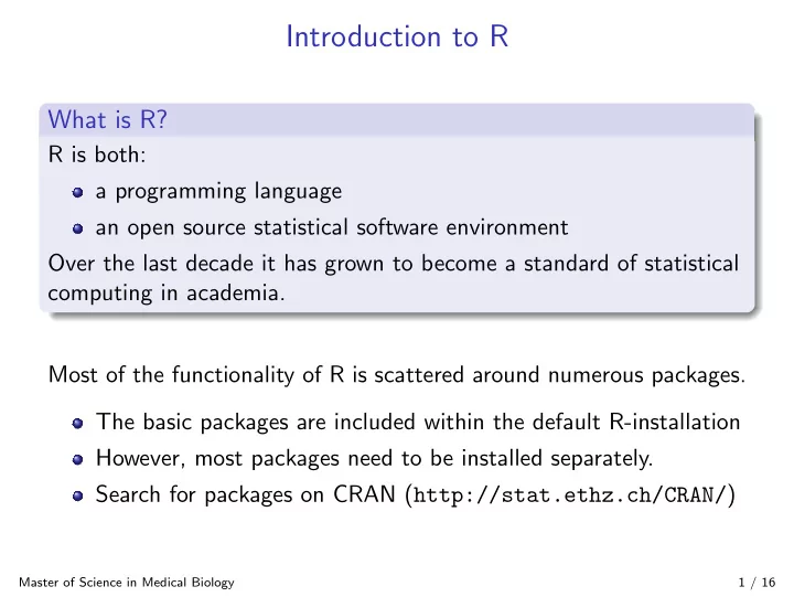
Introduction to R What is R? R is both: a programming language an open source statistical software environment Over the last decade it has grown to become a standard of statistical computing in academia. Most of the functionality of R is scattered around numerous packages. The basic packages are included within the default R-installation However, most packages need to be installed separately. Search for packages on CRAN ( http://stat.ethz.ch/CRAN/ ) Master of Science in Medical Biology 1 / 16
Getting help with functions and features R has an inbuilt help facility. To get more information to any specific named function, for example mean , the command is: > help(mean) or, alternatively: > ?mean If you don’t know the exact name of the function, for example to plot a histogram, use: > help.search("histogram") or, alternatively: > ??histogram Manual: An Introduction to R by Venables, Smith & R Development Core Team (2009). See also > help.start() Master of Science in Medical Biology 2 / 16
Vectors Vectors and assignment: To set up a vector named x , say, consisting of four numbers, namely 1.2, 3.1, 4.8, 5.0, use the R command: > x <- c(1.2, 3.1, 4.8, 5) > a1 <- c(1, 2, 3, 4) > a2 <- 1:4 This is an assignment statement. The assignment operator is < -. The further assignment > y <- c(x, 0, x) creates a vector of length 9 containing two copies of x separated by a zero. To extract the k-th element of vector y type: > y[k] Vector arithmetic: Vectors can be used in arithmetic expressions. Note: Operations are executed element-wise. Master of Science in Medical Biology 3 / 16
Arithmetic operators and functions Elementary arithmetic operators: + , − , ∗ , / and ^ for raising to power. Common arithmetic functions: log, exp, sin, cos, tan, sqrt, min, max, length, sum, prod, mean, median, sd, var, cor, quantile sort ... Logical operators: <, < = , >, > = , == for exact equality, ! = for inequality Master of Science in Medical Biology 4 / 16
Matrices Creation of a matrix: > m <- matrix(1:6,nrow=2, ncol=3) > m [,1] [,2] [,3] [1,] 1 3 5 [2,] 2 4 6 > m[,2] # to get the 2nd column [1] 3 4 > m[1,] # to get the 1st row [1] 1 3 5 > m[2,3] # to get the third element of the 2nd row [1] 6 You can change entries just by assigning new values: > m[, 1] <- c(1.1, 0) > m [,1] [,2] [,3] [1,] 1.1 3 5 [2,] 0.0 4 6 Master of Science in Medical Biology 5 / 16
Matrices Dimension of a matrix: > dim(m) [1] 2 3 To add a new column use cbind , to add a new row use rbind : > cbind(c(101, 7.1),m) [,1] [,2] [,3] [,4] [1,] 101.0 1.1 3 5 [2,] 7.1 0.0 4 6 > rbind(m, c(-1, 0.01, 4)) [,1] [,2] [,3] [1,] 1.1 3.00 5 [2,] 0.0 4.00 6 [3,] -1.0 0.01 4 Master of Science in Medical Biology 6 / 16
Matrix operations If, for example, A and B are matrices of the same size, then > A * B is the matrix of element by element products, while > A %*% B is the matrix product. Transpose the matrix A using > t(A) Get the diagonal elements with: > diag(A) The inverse of A can be computed with: > solve(A) Master of Science in Medical Biology 7 / 16
Functions in R Using functions already implemented in R: Look at the R help of this function: ?functionname Which arguments have to be provided for the function? functionname(argument1, argument1, ...) Writing your own functions: > euklid <- function(argument1, argument2, ...){ + --- calculations + return(results) + } Writing loops: for-loop > for(i in 1:n){ ... } if-loop > if(x==5){ + ... + }else{ + ... + } Master of Science in Medical Biology 8 / 16
Starting to work with data Loading the body height datafile. Here, the data to be loaded is in a table (white-space delimited text file): > data <- read.table("handsize_2006.txt", header=TRUE, sep=" ") The data table is now stored in the object data . We just read in the table from the file handsize 2006.txt . The table had column titles (header=TRUE) and was separated by whitespaces (sep=" ") . To have a look at the first 6 lines, type: > head(data) sex height hand group tutor gender 1 1 168.0 17.5 1 1 f 2 0 183.5 21.0 1 1 m 3 1 170.0 20.0 1 1 f 4 1 159.0 17.0 1 1 f 5 1 165.0 18.0 1 1 f 6 0 180.0 20.0 1 1 m Master of Science in Medical Biology 9 / 16
Accessing the data You can access the columns by their names. To display the column gender , we can use the operator $: > data$gender[1:10] [1] f m f f f m f m m m Levels: f m Frequency tables of a variable can be calculated using table() : > table(data$gender) f m 139 106 There are 139 females and 106 males. Get a summary for body height: > summary(data$height) Min. 1st Qu. Median Mean 3rd Qu. Max. 150.0 165.0 173.0 172.8 180.0 197.0 Master of Science in Medical Biology 10 / 16
Plot Compare the hand length and body height for males and females: > plot(data$hand, data$height, + xlab="Hand length (cm)", ylab="Body height (cm)", + main="Males and females", type="p") Males and females ● ● ● ● ● 190 ● ● ● ● ● ● ● ● ● ● ● ● ● ● ● ● ● ● ● ● ● ● ● ● ● ● ● ● ● ● ● ● ● ● ● ● ● ● ● ● ● ● ● 180 ● ● ● ● ● ● ● Body height (cm) ● ● ● ● ● ● ● ● ● ● ● ● ● ● ● ● ● ● ● ● ● ● ● ● ● ● ● ● ● ● ● ● ● ● ● ● ● ● ● ● ● ● ● ● ● ● ● ● ● ● ● ● ● ● ● ● ● ● ● ● ● ● ● ● ● ● ● ● ● ● ● ● ● ● ● ● ● ● 170 ● ● ● ● ● ● ● ● ● ● ● ● ● ● ● ● ● ● ● ● ● ● ● ● ● ● ● ● ● ● ● ● ● ● ● ● ● ● ● ● ● ● ● ● ● ● ● ● ● ● ● ● ● ● ● ● ● ● ● ● ● ● ● ● ● ● ● ● ● ● ● ● ● ● ● ● ● ● ● ● ● 160 ● ● ● ● ● ● ● ● ● ● ● ● ● ● ● ● ● ● ● ● ● ● ● ● ● ● ● ● 150 ● 16 17 18 19 20 21 22 Hand length (cm) Master of Science in Medical Biology 11 / 16
Bar chart > tab <- table(data$tutor,data$gender) > barplot(tab/sum(tab)*100,beside=T, col=c(1,2,3), + space=c(.1,.8), xlab="", ylab="Percent", xlim=c(0.5,9.5), + legend=1:3, args.legend=list(title=" Tutor ")) 20 Tutor 1 2 3 15 Percent 10 5 0 f m Master of Science in Medical Biology 12 / 16
Histogram > hist(data$height[data$gender=="f"], col=4, xlab="Body height (in cm)", + main="Females",prob=T, right=F) Females 0.06 0.05 0.04 Density 0.03 0.02 0.01 0.00 150 155 160 165 170 175 180 185 Body height (in cm) Master of Science in Medical Biology 13 / 16
Empirical cumulative distribution function > library(Hmisc) # load the library which includes the Ecdf function > Ecdf(data$height[data$gender=="f"], col=1, lwd=2, + main="Empirircal distribution function", + xlab="Body height", ylab="Distribution function") Empirircal distribution function 1.0 0.8 Distribution function 0.6 0.4 0.2 0.0 150 155 160 165 170 175 180 Body height n:139 m:0 Master of Science in Medical Biology 14 / 16
Boxplot > boxplot(height~sex,data=data,names=c("m","f"), + col=5, xlab="Gender", ylab="Height", pch=19) ● 190 180 Height 170 160 150 ● m f Gender Master of Science in Medical Biology 15 / 16
Quitting R To close R use the command: > q() R asks you whether you would like to save the workspace. If you save the workspace a file called .RData , where the workspace is saved, and a file called .Rhistory , where the commands given in the R session are saved, are generated. You can load the workspace and continue working with the datasets and results already generated. Master of Science in Medical Biology 16 / 16
Recommend
More recommend
Explore More Topics
Stay informed with curated content and fresh updates.


![Statistical analysis [ R ] Dani Arribas-Bel & Thomas De Graaff September 5, 2014 Outline](https://c.sambuz.com/817224/statistical-analysis-s.webp)


