Introduction to Nonlinear Statistics and Neural Networks Vladimir - PowerPoint PPT Presentation
Introduction to Nonlinear Statistics and Neural Networks Vladimir Krasnopolsky NCEP/NOAA & ESSIC/UMD http://polar.ncep.noaa.gov/mmab/people/kvladimir.html 3/6/2013 Meto 630; V.Krasnopolsky, "Nonlinear Statistics and NNs" 1
Introduction to Nonlinear Statistics and Neural Networks Vladimir Krasnopolsky NCEP/NOAA & ESSIC/UMD http://polar.ncep.noaa.gov/mmab/people/kvladimir.html 3/6/2013 Meto 630; V.Krasnopolsky, "Nonlinear Statistics and NNs" 1
Outline • Introduction: Regression Analysis • Regression Models (Linear & Nonlinear) • NN Tutorial • Some Atmospheric & Oceanic Applications – Accurate and fast emulations of model physics – NN Multi-Model Ensemble • How to Apply NNs • Conclusions 3/6/2013 Meto 630; V.Krasnopolsky, "Nonlinear Statistics and NNs" 2
Evolution in Statistics Objects Complex, nonlinear, multi-disciplinary, Simple, linear or quasi-linear, single Studied: disciplinary, low-dimensional systems high-dimensional systems 1900 – 1949 1950 – 1999 2000 – … T (years) Tools Simple, linear or quasi-linear, Complex, nonlinear, high-dimensional low-dimensional framework of classical Used: framework… (NNs) statistics (Fischer, about 1930) Under Construction! Teach at the University! • New Paradigm under • Problems for Classical Construction: Paradigm: – Is still quite fragmentary – Nonlinearity & Complexity – Has many different names and gurus – High Dimensionality - – NNs are one of the tools Curse of Dimensionality developed inside this paradigm 3/6/2013 Meto 630; V.Krasnopolsky, "Nonlinear Statistics and NNs" 3
Statistical Inference: A Generic Problem Problem: Information exists in the form of finite sets of values of several related variables (sample or training set) – a part of the population: ℵ = {( x 1 , x 2 , ..., x n ) p , z p } p =1,2,..., N – x 1 , x 2 , ..., x n - independent variables (accurate), – z - response variable (may contain observation errors ε ) We want to find responses z’ q for another set of ℵ′ independent variables = {( x’ 1 , x’ 2 , ..., x’ n ) q } q=1,..,M ℵ′ ∉ ℵ 3/6/2013 Meto 630; V.Krasnopolsky, "Nonlinear Statistics and NNs" 4
Regression Analysis (1): General Solution and Its Limitations Sir Ronald A. Fisher ~ 1930 REGRESSION FUNCTION z = f(X), for all X INDUCTION DEDUCTION Ill-posed problem Well-posed problem DATA: Another Set DATA: Training Set ( x’ 1 , x’ 2 , ..., x’ n ) q =1,2,..., M {( x 1 , x 2 , ..., x n ) p , z p } p =1,2,..., N z q = f(X q ) TRANSDUCTION SVM Find mathematical function f which describes this relationship: 1. Identify the unknown function f 2. Imitate or emulate the unknown function f 3/6/2013 Meto 630; V.Krasnopolsky, "Nonlinear Statistics and NNs" 5
Regression Analysis (2): A Generic Solution • The effect of independent variables on the response is expressed mathematically by the regression or response function f: y = f ( x 1 , x 2 , ..., x n ; a 1 , a 2 , ..., a q ) • y - dependent variable • a 1 , a 2 , ..., a q - regression parameters (unknown!) • f - the form is usually assumed to be known • Regression model for observed response variable: z = y + ε = f ( x 1 , x 2 , ..., x n ; a 1 , a 2 , ..., a q ) + ε • ε - error in observed value z 3/6/2013 Meto 630; V.Krasnopolsky, "Nonlinear Statistics and NNs" 6
Regression Models (1): Maximum Likelihood • Fischer suggested to determine unknown regression parameters { a i } i=1,..,q maximizing the functional: [ ] N Not always!!! = ∑ ρ − = L ( a ) ln ( z y ) ; where y f ( x , a ) p p p p = p 1 here ρ ( ε ) is the probability density function of errors ε i • In a case when ρ ( ε ) is a normal distribution − 2 ( z y ) ρ − = α ⋅ − ( z y ) exp( ) σ 2 the maximum likelihood => least squares ⎡ ⎤ − 2 ( z y ) N N ∑ ∑ p p = α ⋅ − = − ⋅ − 2 L ( a ) ln ⎢ exp( ) ⎥ A B ( z y ) σ p p 2 ⎢ ⎥ ⎣ ⎦ = = p 1 p 1 N ∑ ⇒ − 2 max L min ( z y ) p p = p 1 3/6/2013 Meto 630; V.Krasnopolsky, "Nonlinear Statistics and NNs" 7
Regression Models (2): Method of Least Squares • To find unknown regression parameters {a i } i=1,2,...,q , the method of least squares can be applied: N N ∑ ∑ = − 2 = − 2 E a a ( , ,..., a ) ( z y ) [ z f (( x ,..., x ) ; a a , ,..., a )] 1 2 q p p p 1 n p 1 2 q = = p 1 p 1 • E ( a 1 ,..., a q ) - error function = the sum of squared deviations. • To estimate {a i } i=1,2,...,q => minimize E => solve the system of equations: ∂ E = = 0 ; i 12 , ,..., q ∂ a i • Linear and nonlinear cases. 3/6/2013 Meto 630; V.Krasnopolsky, "Nonlinear Statistics and NNs" 8
Regression Models (3): Examples of Linear Regressions • Simple Linear Regression: z = a 0 + a 1 x 1 + ε • Multiple Linear Regression: n ∑ + + ε a a x z = a 0 + a 1 x 1 + a 2 x 2 + ... + ε = 0 i i = i 1 • Generalized Linear Regression: n ∑ + + ε a a f x ( ) z = a 0 + a 1 f 1 (x 1 )+ a 2 f 2 (x 2 ) + ... + ε = 0 i i i = i 1 – Polynomial regression, f i (x) = x i , No free z = a 0 + a 1 x+ a 2 x 2 + a 3 x 3 + ... + ε parameters – Trigonometric regression, f i (x) = cos(ix) z = a 0 + a 1 cos(x) + a 1 cos(2 x) + ... + ε 3/6/2013 Meto 630; V.Krasnopolsky, "Nonlinear Statistics and NNs" 9
Regression Models (4): Examples of Nonlinear Regressions • Response Transformation Regression: G(z) = a 0 + a 1 x 1 + ε • Example: z = exp(a 0 + a 1 x 1 ) G(z) = ln(z) = a 0 + a 1 x 1 Free • Projection-Pursuit Regression: nonlinear k n parameters ∑ ∑ = + Ω y a a f ( x ) 0 j ji i = = j 1 i 1 • Example: k n ∑ ∑ = + + Ω + ε z a a tanh( b x ) 0 j j ji i = = j 1 i 1 3/6/2013 Meto 630; V.Krasnopolsky, "Nonlinear Statistics and NNs" 10
NN Tutorial: Introduction to Artificial NNs • NNs as Continuous Input/Output Mappings – Continuous Mappings: definition and some examples – NN Building Blocks: neurons, activation functions, layers – Some Important Theorems • NN Training • Major Advantages of NNs • Some Problems of Nonlinear Approaches 3/6/2013 Meto 630; V.Krasnopolsky, "Nonlinear Statistics and NNs" 11
Mapping Generalization of Function • Mapping: A rule of correspondence established between vectors in vector ℜ ℜ spaces and that associates each n m ℜ n vector X of a vector space with a vector Y in another vector space . ℜ m = ⎡ ⎤ y f ( x , x ,..., x ) = ⎫ 1 1 1 2 n Y F ( X ) ⎢ ⎥ = ⎪ y f ( x , x ,..., x ) ⎢ ⎥ = ∈ ℜ ≠ 2 2 1 2 n n X { x , x ,..., x }, ⎬ ⎢ ⎥ 1 2 n ⎪ ⎢ ⎥ = ∈ ℜ m Y { y , y ,..., y }, ⎭ = 1 2 m y f ( x , x ,..., x ) ⎣ ⎦ m m 1 2 n 3/6/2013 Meto 630; V.Krasnopolsky, "Nonlinear Statistics and NNs" 12
Mapping Y = F ( X ): examples • Time series prediction: X = { x t , x t-1 , x t-2 , ..., x t-n }, - Lag vector Y = { x t+1 , x t+2 , ..., x t+m } - Prediction vector (Weigend & Gershenfeld, “Time series prediction”, 1994) • Calculation of precipitation climatology: X = { Cloud parameters, Atmospheric parameters } Y = { Precipitation climatology } (Kondragunta & Gruber, 1998) • Retrieving surface wind speed over the ocean from satellite data (SSM/I): X = { SSM/I brightness temperatures } Y = { W , V , L , SST } (Krasnopolsky, et al., 1999; operational since 1998) • Calculation of long wave atmospheric radiation: X = { Temperature, moisture, O 3 , CO 2 , cloud parameters profiles, surface fluxes, etc .} Y = { Heating rates profile, radiation fluxes } (Krasnopolsky et al., 2005) 3/6/2013 Meto 630; V.Krasnopolsky, "Nonlinear Statistics and NNs" 13
NN - Continuous Input to Output Mapping Multilayer Perceptron: Feed Forward, Fully Connected Linear Nonlinear x Neurons Neurons Neuron 1 x 1 t y 1 1 x 2 x 2 t j Linear Part Nonlinear Part y 2 x b j · X + b 0 = s j � (s j ) = t j x 3 3 X t y Y x 3 2 4 x n n ∑ t = φ + ⋅ = t ( b b x ) k y j j 0 ji i m = i 1 x n ∑ n Output = + ⋅ tanh( b b x ) Hidden Input j 0 ji i Layer Layer = i 1 Layer ⎧ k k n ∑ ∑ ∑ = + ⋅ = + ⋅ φ + ⋅ = y a a t a a ( b b x ) ⎪ q q 0 qj j q 0 qj j 0 ji i ⎪ = = = j 1 j 1 i 1 Y = F NN (X) ⎨ k n ⎪ ∑ ∑ Jacobian ! = + ⋅ + ⋅ = a a tanh( b b x ); q 1 , 2 ,..., m ⎪ q 0 qj j 0 ji i ⎩ = = j 1 i 1 3/6/2013 Meto 630; V.Krasnopolsky, "Nonlinear Statistics and NNs" 14
Some Popular Activation Functions tanh(x) Sigmoid, (1 + exp(-x)) -1 X X Hard Limiter Ramp Function X X 3/6/2013 Meto 630; V.Krasnopolsky, "Nonlinear Statistics and NNs" 15
NN as a Universal Tool for Approximation of Continuous & Almost Continuous Mappings Some Basic Theorems: Any function or mapping Z = F (X), continuous on � a compact subset, can be approximately represented by a p (p � 3) layer NN in the sense of uniform convergence (e.g., Chen & Chen, 1995; Blum and Li, 1991, Hornik, 1991; Funahashi, 1989, etc.) The error bounds for the uniform approximation � on compact sets (Attali & Pagès, 1997): ||Z -Y|| = ||F (X) - F NN (X)|| ~ C/k k -number of neurons in the hidden layer C – does not depend on n (avoiding Curse of Dimensionality!) 3/6/2013 Meto 630; V.Krasnopolsky, "Nonlinear Statistics and NNs" 16
Recommend
More recommend
Explore More Topics
Stay informed with curated content and fresh updates.
