Introduction to Matlab Marco Chiarandini Department of Mathematics - PowerPoint PPT Presentation

FF505/FY505 Computational Science Lecture 1 Introduction to Matlab Marco Chiarandini Department of Mathematics & Computer Science University of Southern Denmark

Course Organization Overview of MATLAB Outline Solving Linear Systems 1. Course Organization 2. Overview of MATLAB 3. Solving Linear Systems 2

Course Organization Overview of MATLAB Outline Solving Linear Systems 1. Course Organization 2. Overview of MATLAB 3. Solving Linear Systems 3

Course Organization Overview of MATLAB On the Course Solving Linear Systems Organization 1. Introduction to mathematical tools (Claudio) – weeks 5-8 2. Tutorial on numerical software, MATLAB (Marco) – weeks 5-8 3. Laboratories on applications in physics (Paolo) – weeks 7-11 Evaluation Group project during the laboratory session + oral exam 4

Course Organization Overview of MATLAB MATLAB Section Solving Linear Systems The MATLAB Section will cover MATLAB interactive environment MATLAB vectorized operations MATLAB programming data input/output simple visualization. More specifically, it should prepare you to carry out the exercises from the theory and laboratory sections. 5

Course Organization Overview of MATLAB MATLAB Section – Schedule Solving Linear Systems Schedule for weeks 5-8 (4 weeks): Lecture, Thursday, 10:15-12:00, U140, (weeks 05-08) Tutorials: S1 (FF505/FY505), Thursday, 12-14 U10 (weeks 05-08) S6 (FF505), Friday, 12-14, U14, (week 05) S6 (FF505), Friday, 08-10, U14 (weeks 06-08) S9 (FY505), Friday, 10-12, U49c (weeks 05-08) From week 7 you’ll start also laboratories 6

Course Organization Overview of MATLAB Solving Linear Systems Communication tools BlackBoard (BB) (link to MATLAB Section http://www.imada.sdu.dk/~marco/FF505 ) Announcements in BlackBoard Personal email of instructors and Marco Ask peers 7

Course Organization Overview of MATLAB Hands on Experience Solving Linear Systems Weekly exercises to be carried out in your study group outside of tutorial sessions. Slides and exercises sheets are posted after lecture at http://www.imada.sdu.dk/~marco/FF505 Getting MATLAB machines in IMADA terminal room and in U26B (12 PCs) (type matlab from command line) use a Matlab clone, eg, Octave buy the student edition of Matlab: 89$ (ca. 500 DDK) Link: http://www.mathworks.se/academia/student_version/ Then click on “BUY NOW” 8

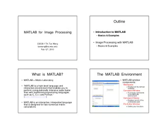
Course Organization Overview of MATLAB MATLAB Solving Linear Systems MATLAB ( ma trix la boratory) is a high-level language and interactive environment to perform computationally intensive numerical computations faster than with low-level programming languages such as C, C++, and Fortran. Developed by a privately held company, MathWorks, 70% located at the company’s headquarters in Massachusetts. Stable release: 2012b (we have 2008b) Written in C, Java License: Proprietary 9

Course Organization Overview of MATLAB Scientific vs Symbolic Computing Solving Linear Systems scientific computing is based on numerical computation with approximate floating point numbers. symbolic computation manipulates mathematical expressions and other mathematical objects. emphasis on exact computation with expressions containing variables that have not any given value and are thus manipulated as symbols � Try http://www.wolframalpha.com Symbolic computation can be done in MATLAB with the Symbolic Math Toolbox and the MuPAD editor (not installed) 10

Course Organization Overview of MATLAB Solving Linear Systems Other similar numerical computing environments with high-level programming language are: Maple www.maplesoft.com (symbolic) – Proprietary Mathematica http://www.wolfram.com/mathematica (discrete mathematics) – [Proprietary] Octave www.gnu.org/software/octave – [General Public License] R www.r-project.org (statistics) – [GPL] Sage www.sagemath.org (discrete mathematics) – [GPL] SciPy www.scipy.org (based on python) – [GPL] ... 11

Course Organization Overview of MATLAB Outline Solving Linear Systems 1. Course Organization 2. Overview of MATLAB 3. Solving Linear Systems 12

Course Organization Overview of MATLAB MATLAB Desktop Solving Linear Systems Command line programming Command window ✞ ☎ Workspace %%% elementary operations 5+6 Command history 3-2 5*8 Current folder browser 1/2 2^6 1 == 2 % false Variable editor 1 ~= 2 % true. note, not "!=" 1 && 0 MATLAB program editor 1 || 0 xor(1,0) ✝ ✆ Help Desktop menu Docking/Undocking, maximize by double click Current folder Search path ( File menu -> set path ) 13

Course Organization Overview of MATLAB Variable Assignment Solving Linear Systems The = sign in MATLAB represents the assignment or replacement operator. It has a different meaning than in mathematics. Compare: x = x + 3 In math it implies 0=2, which is an invalid statement In MATLAB it adds 2 to the current value of the variable ✞ ☎ ✞ ☎ %% variable assignment x + 2 = 20 % wrong statement a = 3; % semicolon suppresses output x = 5 + y % wrong if y unassigned ✝ ✆ b = ’hi’; c = 3>=1; Variables are visible in the workspace % Displaying them: Names: a = pi disp(sprintf(’2 decimals: %0.2f’, a)) [a-z][A-Z][0-9]_ disp(sprintf(’6 decimals: %0.6f’, a)) format long % 16 decimal digits case sensitive a format short e % 4 decimal digits + max 63 chars scientific notation a ✝ ✆ 14

Course Organization Overview of MATLAB Managing the Work Session Solving Linear Systems ✞ ☎ Predefined variables who % lists variables currently in memory ✞ ☎ whos % lists current variables and sizes pi clear v % clear w/ no argt clears all Inf % 5/0 edit filename % edit a script file NaN % 0/0 clc % clears theCommand window eps % accuracy of computations ... % ellipsis; continues a line i,j % immaginary unit i=j=sqrt( − 1) help rand % returns help of a function 3+8i % a complex number (no ∗ ) quit % stops MATLAB Complex(1,-2) ✝ ✆ ✝ ✆ 15

Course Organization Overview of MATLAB Working with Files Solving Linear Systems MATLAB handles three types of files: M-files .m : Function and program files MAT-files .mat : binary files with name and values of variables data file .dat : ASCII files ✞ ☎ %% loading data load q1y.dat load q1x.dat save hello v; % save variable v into file hello.mat save hello.txt v -ascii; % save as ascii % fopen, fprintf, fscanf also work % ls %% cd, pwd & other unix commands work in matlab; % to access shell, preface with "!" ✝ ✆ Files are stored and search in current directory and search path 16

Course Organization Overview of MATLAB Directories and paths Solving Linear Systems If we type problem1 1. seeks if it is a variable and displays its value 2. checks if it is one of its own programs and executes it 3. looks in the current directory for file program1.m and executes the file 4. looks in the search path for file program1.m and executes it ✞ ☎ addpath dirname % adds the directory dirname to the search path cd dirname % changes the current directory to dirname dir % lists all files in the current directory dir dirname % lists all files in dirname path % displays the MATLAB search path pathtool % starts the Set Path tool pwd % displays the current directory rmpath dirname % removes the directory dirname from the search path what % lists MATLAB specific files in the current directory what dirname % lists MATLAB specific files in dirname which item % displays the path name of item ✝ ✆ 17

Course Organization Overview of MATLAB Arrays and Matrices Solving Linear Systems Arrays are the basic data structures of MATLAB Types of arrays: numeric • character • logical • cell • structure • function handle ✞ ☎ %% vectors and matrices A = [1 2; 3 4; 5 6] v = [1 2 3] v = [1; 2; 3] v = [1:0.1:2] % from 1 to 2, with stepsize of 0.1. Useful for plot axes v = 1:6 % from 1 to 6, assumes stepsize of 1 C = 2*ones(2,3) % same as C = [2 2 2; 2 2 2] w = ones(1,3) % 1x3 vector of ones w = zeros(1,3) w = rand(1,3) % drawn from a uniform distribution w = randn(1,3) % drawn from a normal distribution (mean=0, var=1) w = -6 + sqrt(10)*(randn(1,10000)) % (mean = 1, var = 2) hist(w) % histogram e = []; % empty vector I = eye(4) % 4x4 identity matrix A = linspace(5,8,31) % equivalent to 5:0.1:8 ✝ ✆ 18

Course Organization Overview of MATLAB Solving Linear Systems ✞ ☎ %% indexing A(3,2) % indexing is (row,col) A(2,:) % get the 2nd row. %% ":" means every elt along that dimension A(:,2) % get the 2nd col A(1,end) % 1st row, last elt. Indexing starts from 1. A(end,:) % last row A([1 3],:) = [] % deletes 1st and 3rd rows A(:,2) = [10 11 12]’ % change second column A = [A, [100; 101; 102]]; % append column vec % A = [ones(size(A,1),1), A]; % e.g bias term in linear regression A(:) % Select all elements as a column vector. ✝ ✆ ✞ ☎ %% dimensions sz = size(A) size(A,1) % number of rows size(A,2) % number of cols length(v) % size of longest dimension ✝ ✆ 19

Course Organization Overview of MATLAB Matrix Operations Solving Linear Systems ✞ ☎ %% matrix operations A * C % matrix multiplication B = [5 6; 7 8; 9 10] % same dims as A A .* B % element − wise multiplcation % A . ∗ C or A ∗ B gives error − wrong dimensions A .^ 2 1./v log(v) % functions like this operate element − wise on vecs or matrices exp(v) % e^4 abs(v) -v % − 1 ∗ v v + ones(1,length(v)) % v + 1 % same A’ % (conjuate) transpose ✝ ✆ 20