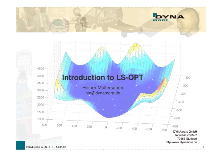
Introduction to LS-OPT Heiner Mllerschn hm@dynamore.de DYNA more - PowerPoint PPT Presentation
Introduction to LS-OPT Heiner Mllerschn hm@dynamore.de DYNA more GmbH Industriestrae 2 70565 Stuttgart http://www.dynamore.de Introduction to LS-OPT 14.05.08 1 Overview n Introduction/Features n Methodologies Optimization n
Introduction to LS-OPT Heiner Müllerschön hm@dynamore.de DYNA more GmbH Industriestraße 2 70565 Stuttgart http://www.dynamore.de Introduction to LS-OPT – 14.05.08 1
Ł Overview n Introduction/Features n Methodologies – Optimization n Methodologies - Robustness n Examples - Optimization n Examples - Robustness n Version 3.3 / Outlook Introduction to LS-OPT – 14.05.08 2
§ Introduction/Features § Methods – Optimization § Methods - Robustness Introduction / Features § Examples - Optimization § Examples - Robustness § Version 3.3 / Outlook Ł About LS-OPT � LS-OPT is a product of LSTC (Livermore Software Technology Corporation) � LS-OPT can be linked to any simulation code – stand alone optimization software � Methodologies/Features: � Successive Response Surface Method (SRSM) � Genetic Algorithm (MOGA->NSGA-II) � Multidisciplinary optimization (MDO) � Multi-Objective optimization (Pareto) � numerical/analytical based sensitivities � Analysis of Variance (ANOVA) � Stochastic/Probabilistic Analysis � Monte Carlo Analysis using Metamodels � …. Introduction to LS-OPT – 14.05.08 3
§ Introduction/Features § Methods – Optimization § Methods - Robustness Introduction / Features § Examples - Optimization § Examples - Robustness § Version 3.3 / Outlook Ł About LS-OPT � Mixed Discrete-Continous Optimization � Specify sets of discrete variables (e.g. sheet thicknesses) � Robust Parameter Design (RDO) � Improve/Maximizing the robustness of the optimum � Reliability Based Design Optimization (RBDO) � Improve failure probability of optimum � Visualization of Stochastic Results � Confidence Intervals, reliability quantities � Fringe of statistic results on the FE-Model Introduction to LS-OPT – 14.05.08 4
§ Introduction/Features § Methods – Optimization § Methods - Robustness Introduction / Features § Examples - Optimization § Examples - Robustness § Version 3.3 / Outlook Ł About LS-OPT � Job Distribution - Interface to Queuing Systems � PBS, LSF, LoadLeveler, SLURM, AQS, etc. � Retry of failed queuing (abnormal termination) � LS-OPT might be used as a “Process Manager” � Shape Optimization � Interface to ANSA , HyperMorph, DEP-Morpher, SFE-Concept � User-defined interface to any Pre-Processor Introduction to LS-OPT – 14.05.08 5
§ Introduction/Features § Methods – Optimization § Methods - Robustness Introduction / Features § Examples - Optimization § Examples - Robustness § Version 3.3 / Outlook Ł About LS-OPT � LS-DYNA Integration � Checking of Dyna keyword files (*DATABASE_) � Importation of design parameters from Dyna keyword files (*PARAMETER_) � Monitoring of LS-DYNA progress � Result extraction of most LS-DYNA response types � D3plot compression (node and part selection) Introduction to LS-OPT – 14.05.08 6
§ Introduction/Features § Methods – Optimization § Methods - Robustness Introduction / Features § Examples - Optimization § Examples - Robustness § Version 3.3 / Outlook Ł About LS-OPT � Parameter Identification Module 2 1 ∑ − ( ) F G P � Handles "continuous" test curves x i i W i P s = p 1 � Automated use of test results to i calibrate materials/systems � Simplify input for system identification applications � Visualization of test and simulation curve to compare � Confidence intervals for individual parameters in parameter identification Introduction to LS-OPT – 14.05.08 7
§ Introduction/Features § Methods – Optimization § Methods - Robustness Methods - Optimization § Examples - Optimization § Examples - Robustness § Version 3.3 / Outlook Ł Response Surface Methodology - Optimization Process Response Objective values 1 e l b a i r a V Response n g i s e surface D Design space Experimental Subregion Design points (Range) D e s i g Starting (base) n V a r i a design b l e 2 Introduction to LS-OPT – 14.05.08 8
§ Introduction/Features § Methods – Optimization § Methods - Robustness Methods - Optimization § Examples - Optimization § Examples - Robustness § Version 3.3 / Outlook Ł Find an Optimum on the Response Surface (one iteration) Starting value on response surface Optimization of sub-problem (response surface) using LFOPC algorithm Optimum ( predicted by response surface) Optimum ( computed by simulation using design variables) Introduction to LS-OPT – 14.05.08 9
§ Introduction/Features § Methods – Optimization § Methods - Robustness Methods - Optimization § Examples - Optimization § Examples - Robustness § Version 3.3 / Outlook Ł Successive Response Surface Methodology Design Variable 2 Region of Interest optimum Design Space Design Variable 1 Introduction to LS-OPT – 14.05.08 10
§ Introduction/Features § Methods – Optimization § Methods - Robustness Methods - Optimization § Examples - Optimization § Examples - Robustness § Version 3.3 / Outlook Ł Successive Response Surface Methodology � Example - 4th order polynomial 9 = + − + + − + − 2 2 4 2 g ( ) 4 x 4 x x 2 x 2 x x x 2 x x x 1 2 1 2 1 2 1 1 2 2 movie Introduction to LS-OPT – 14.05.08 11
§ Introduction/Features § Methods – Optimization § Methods - Robustness Methods - Optimization § Examples - Optimization § Examples - Robustness § Version 3.3 / Outlook Ł Design of Experiments (DOE) - Sampling Point Selection � Koshal, Central Composite, Full Factorial � D-Optimality Criterion - Gives maximal confidence in the model T max X X � Monte Carlo Sampling � Latin Hypercube Sampling (stratified Monte Carlo) � Space Filling Designs � User Defined Experiments Introduction to LS-OPT – 14.05.08 12
§ Introduction/Features § Methods – Optimization § Methods - Robustness Methods - Optimization § Examples - Optimization § Examples - Robustness § Version 3.2 / Outlook Ł Response Surfaces (Meta Models) � Linear, Quadratic and Mixed polynomial based � Neural Network and Kriging for Nonlinear Regression linear polynomial quadratic polynomial neural network Introduction to LS-OPT – 14.05.08 13
§ Introduction/Features § Methods – Optimization § Methods - Robustness Methods - Optimization § Examples - Optimization § Examples - Robustness § Version 3.2 / Outlook Ł Neural Network Regression � Example - 4th order polynomial 9 = + − + + − + − 2 2 4 2 g ( ) 4 x 4 x x 2 x 2 x x x 2 x x x 1 2 1 2 1 2 1 1 2 2 analytical function (green) global neural net approx. with 20 points (red) simulation points movie Introduction to LS-OPT – 14.05.08 14
§ Introduction/Features § Methods – Optimization Exploring Design Space § Methods - Robustness § Examples - Optimization using D-SPEX § Examples - Robustness § Version 3.2 / Outlook Ł Meta-Model Viewer - Exploration of Design Space n Compare responses, histories or even different optimization projects Introduction to LS-OPT – 14.05.08 15
§ Introduction/Features § Methods – Optimization Exploring Design Space § Methods - Robustness § Examples - Optimization using D-SPEX § Examples - Robustness § Version 3.2 / Outlook Ł About D-SPEX � D-SPEX – D esign SP ace EX plorer � D-SPEX is a software tool for the visualization of Meta-Models and results of optimization or stochastic analysis � Versions Windows 32/64bit and Linux 32/64bit � Complete interface to LS-OPT database � Developed by DYNA more in collaboration with AUDI (property of DYNAmore) feasible � Methodologies/Features: � Meta-Model viewer � Curve statistics � Feasible/Infeasible design � Ant-Hill plots � Statistic evaluations optimum on response surface Introduction to LS-OPT – 14.05.08 16
§ Introduction/Features § Methods – Optimization § Methods - Robustness Methods - Optimization § Examples - Optimization § Examples - Robustness § Version 3.2 / Outlook Ł Overview – Optimization Methodologies for highly nonlinear Applications Gradient Based Random Search Genetic RSM / SRSM Methods Algorithms § accuracy of § very robust, can not § good for problems § very effective, solution diverge with many local particularly SRSM minimas § number of solver § easy to apply § trade-off studies calls on RS § filter out noise, smoothing of results § can diverge § bad convergence, § many solver calls, § approximation not effective only suitable for fast error § can stuck in local solver runs minimas § Chooses best § verification run observation – § Chooses best might be infeasible § step-size may not be observation – dilemma for § number of representative of a may not be numerical gradients variables control good (robust) design representative of a minimum number of good (robust) design required runs Introduction to LS-OPT – 14.05.08 17
Recommend
More recommend
Explore More Topics
Stay informed with curated content and fresh updates.

