Introduction to Artificial Intelligence Belief networks Chapter - PowerPoint PPT Presentation
Introduction to Artificial Intelligence Belief networks Chapter 15.12 Dieter Fox Based on AIMA Slides S. Russell and P. Norvig, 1998 c Chapter 15.12 0-0 Outline Bayesian networks: syntax and semantics Inference tasks Based
Introduction to Artificial Intelligence Belief networks Chapter 15.1–2 Dieter Fox Based on AIMA Slides � S. Russell and P. Norvig, 1998 c Chapter 15.1–2 0-0
Outline ♦ Bayesian networks: syntax and semantics ♦ Inference tasks Based on AIMA Slides � S. Russell and P. Norvig, 1998 c Chapter 15.1–2 0-1
Belief networks A simple, graphical notation for conditional independence assertions and hence for compact specification of full joint distributions Syntax: a set of nodes, one per variable a directed, acyclic graph (link ≈ “directly influences”) a conditional distribution for each node given its parents: P ( X i | Parents ( X i )) In the simplest case, conditional distribution represented as a conditional probability table (CPT) Based on AIMA Slides � S. Russell and P. Norvig, 1998 c Chapter 15.1–2 0-2
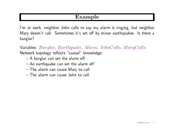
✁ � ✁ � ✂ ✁ ✄ ✁ � � ✁ � � ✁ Example I’m at work, neighbor John calls to say my alarm is ringing, but neighbor Mary doesn’t call. Sometimes it’s set off by minor earthquakes. Is there a burglar? Variables: Burglar , Earthquake , Alarm , JohnCalls , MaryCalls Network topology reflects “causal” knowledge: P(E) P(B) Burglary Earthquake .002 .001 B E P(A) T T .95 Alarm T F .94 F T .29 F F .001 A P(J) A P(M) T .90 JohnCalls T .70 MaryCalls F .05 F .01 Based on AIMA Slides � S. Russell and P. Norvig, 1998 c Chapter 15.1–2 0-3
✁ � ✁ � ✂ ✁ ✄ ✁ � � ✁ � � ✁ Example I’m at work, neighbor John calls to say my alarm is ringing, but neighbor Mary doesn’t call. Sometimes it’s set off by minor earthquakes. Is there a burglar? Variables: Burglar , Earthquake , Alarm , JohnCalls , MaryCalls Network topology reflects “causal” knowledge: P(E) P(B) Burglary Earthquake .002 .001 B E P(A) T T .95 Alarm T F .94 F T .29 F F .001 A P(J) A P(M) T .90 JohnCalls T .70 MaryCalls F .05 F .01 Note: ≤ k parents ⇒ O ( d k n ) numbers vs. O ( d n ) Based on AIMA Slides � S. Russell and P. Norvig, 1998 c Chapter 15.1–2 0-4
Semantics “Global” semantics defines the full joint distribution as the product of the local conditional distributions: n P ( X 1 , . . . , X n ) = Π i = 1 P ( X i | Parents ( X i )) e.g., P ( J ∧ M ∧ A ∧ ¬ B ∧ ¬ E ) is given by ?? = Based on AIMA Slides � S. Russell and P. Norvig, 1998 c Chapter 15.1–2 0-5
Semantics “Global” semantics defines the full joint distribution as the product of the local conditional distributions: n P ( X 1 , . . . , X n ) = Π i = 1 P ( X i | Parents ( X i )) e.g., P ( J ∧ M ∧ A ∧ ¬ B ∧ ¬ E ) is given by ?? = P ( ¬ B ) P ( ¬ E ) P ( A |¬ B ∧ ¬ E ) P ( J | A ) P ( M | A ) “Local” semantics: each node is conditionally independent of its nondescendants given its parents Theorem: Local semantics ⇔ global semantics Based on AIMA Slides � S. Russell and P. Norvig, 1998 c Chapter 15.1–2 0-6
Markov blanket Each node is conditionally independent of all others given its Markov blanket : parents + children + children’s parents U 1 U m . . . X Z 1j Z nj Y Y n 1 . . . Based on AIMA Slides � S. Russell and P. Norvig, 1998 c Chapter 15.1–2 0-7
Constructing belief networks Need a method such that a series of locally testable assertions of conditional independence guarantees the required global semantics 1. Choose an ordering of variables X 1 , . . . , X n 2. For i = 1 to n add X i to the network select parents from X 1 , . . . , X i − 1 such that P ( X i | Parents ( X i )) = P ( X i | X 1 , . . . , X i − 1 ) This choice of parents guarantees the global semantics: n P ( X 1 , . . . , X n ) = Π i = 1 P ( X i | X 1 , . . . , X i − 1 ) (chain rule) n = Π i = 1 P ( X i | Parents ( X i )) by construction Based on AIMA Slides � S. Russell and P. Norvig, 1998 c Chapter 15.1–2 0-8
� Example Suppose we choose the ordering M , J , A , B , E MaryCalls JohnCalls P ( J | M ) = P ( J ) ? Based on AIMA Slides � S. Russell and P. Norvig, 1998 c Chapter 15.1–2 0-9
✁ � Example Suppose we choose the ordering M , J , A , B , E MaryCalls JohnCalls Alarm P ( J | M ) = P ( J ) ? No P ( A | J, M ) = P ( A | J ) ? P ( A | J, M ) = P ( A ) ? Based on AIMA Slides � S. Russell and P. Norvig, 1998 c Chapter 15.1–2 0-10
� ✁ Example Suppose we choose the ordering M , J , A , B , E MaryCalls JohnCalls Alarm Burglary P ( J | M ) = P ( J ) ? No P ( A | J, M ) = P ( A | J ) ? P ( A | J, M ) = P ( A ) ? No P ( B | A, J, M ) = P ( B | A ) ? P ( B | A, J, M ) = P ( B ) ? Based on AIMA Slides � S. Russell and P. Norvig, 1998 c Chapter 15.1–2 0-11
✁ � Example Suppose we choose the ordering M , J , A , B , E MaryCalls JohnCalls Alarm Burglary Earthquake P ( J | M ) = P ( J ) ? No P ( A | J, M ) = P ( A | J ) ? P ( A | J, M ) = P ( A ) ? No P ( B | A, J, M ) = P ( B | A ) ? Yes P ( B | A, J, M ) = P ( B ) ? No P ( E | B, A, J, M ) = P ( E | A ) ? P ( E | B, A, J, M ) = P ( E | A, B ) ? Based on AIMA Slides � S. Russell and P. Norvig, 1998 c Chapter 15.1–2 0-12
✁ � Example Suppose we choose the ordering M , J , A , B , E MaryCalls JohnCalls Alarm Burglary Earthquake P ( J | M ) = P ( J ) ? No P ( A | J, M ) = P ( A | J ) ? P ( A | J, M ) = P ( A ) ? No P ( B | A, J, M ) = P ( B | A ) ? Yes P ( B | A, J, M ) = P ( B ) ? No P ( E | B, A, J, M ) = P ( E | A ) ? No P ( E | B, A, J, M ) = P ( E | A, B ) ? Yes Based on AIMA Slides � S. Russell and P. Norvig, 1998 c Chapter 15.1–2 0-13
✁ ✁ ✂ ✁ ✂ � Example: Car diagnosis Initial evidence: engine won’t start Testable variables (thin ovals), diagnosis variables (thick ovals) Hidden variables (shaded) ensure sparse structure, reduce parameters fanbelt alternator battery age broken broken battery no charging dead fuel line starter battery no oil no gas blocked broken flat engine won’t gas gauge oil light lights start Based on AIMA Slides � S. Russell and P. Norvig, 1998 c Chapter 15.1–2 0-14
Example: Car insurance Predict claim costs (medical, liability, property) given data on application form (other unshaded nodes) SocioEcon Age GoodStudent ExtraCar Mileage RiskAversion VehicleYear SeniorTrain DrivingSkill MakeModel DrivingHist Antilock DrivQuality AntiTheft HomeBase CarValue Airbag Accident Ruggedness Theft OwnDamage Cushioning OwnCost OtherCost MedicalCost LiabilityCost PropertyCost Based on AIMA Slides � S. Russell and P. Norvig, 1998 c Chapter 15.1–2 0-15
Inference in Bayesian networks Instantiate some nodes (evidence nodes) and query other nodes. P ( Burglary | JohnCalls ) ?? Based on AIMA Slides � S. Russell and P. Norvig, 1998 c Chapter 15.1–2 0-16
Inference in Bayesian networks Instantiate some nodes (evidence nodes) and query other nodes. P ( Burglary | JohnCalls ) ?? • Burglary only every 1000 days, but John calls 50 times in 1000 days, i.e. for each burglary we receive 50 false alarms. � P ( Burglary | JohnCalls ) = 0 . 016 ! • P ( Burglary | JohnCalls , MaryCalls ) = 0 . 29 . Based on AIMA Slides � S. Russell and P. Norvig, 1998 c Chapter 15.1–2 0-17
Types of inference 1. Diagnostic : From effects to causes P ( Burglary | JohnCalls ) = 0 . 016 2. Causal : From causes to effects P ( JohnCalls | Burglary ) = 0 . 86 3. Intercausal : between causes of common effect P ( Burglary | Alarm ) = 0 . 376 , but P ( Burglary | Alarm , Earthquake ) = 0 . 003 . 4. Mixed: Combinations of 1.-3. P ( Alarm | JohnCalls , ¬ Earthquake ) = 0 . 03 Based on AIMA Slides � S. Russell and P. Norvig, 1998 c Chapter 15.1–2 0-18
Inference tasks Queries : compute posterior marginal P ( X i | E = e ) e.g., P ( NoGas | Gauge = empty, Lights = on, Starts = false ) Optimal decisions : decision networks include utility information; probabilistic inference required for P ( outcome | action, evidence ) Value of information : which evidence to seek next? Sensitivity analysis : which probability values are most critical? Explanation : why do I need a new starter motor? Based on AIMA Slides � S. Russell and P. Norvig, 1998 c Chapter 15.1–2 0-19
Compact conditional distributions CPT grows exponentially with no. of parents CPT becomes infinite with continuous-valued parent or child Solution: canonical distributions that are defined compactly Deterministic nodes are the simplest case: X = f ( Parents ( X )) for some function f E.g., Boolean functions NorthAmerican ⇔ Canadian ∨ US ∨ Mexican E.g., numerical relationships among continuous variables ∂Level = inflow + precipation - outflow - evaporation ∂t Based on AIMA Slides � S. Russell and P. Norvig, 1998 c Chapter 15.1–2 0-20
Compact conditional distributions contd. Noisy-OR distributions model multiple noninteracting causes 1) Parents U 1 . . . U k include all causes (can add leak node ) 2) Independent failure probability q i for each cause alone j ⇒ P ( X | U 1 . . . U j , ¬ U j +1 . . . ¬ U k ) = 1 − Π i = 1 q i P ( Fever ) P ( ¬ Fever ) Cold Flu Malaria F F F 1 . 0 0.0 F F T 0 . 9 0.1 0 . 8 F T F 0.2 F T T 0 . 98 0 . 02 = 0 . 2 × 0 . 1 T F F 0 . 4 0.6 T F T 0 . 94 0 . 06 = 0 . 6 × 0 . 1 0 . 88 0 . 12 = 0 . 6 × 0 . 2 T T F T T T 0 . 988 0 . 012 = 0 . 6 × 0 . 2 × 0 . 1 Number of parameters linear in number of parents Based on AIMA Slides � S. Russell and P. Norvig, 1998 c Chapter 15.1–2 0-21
Recommend
More recommend
Explore More Topics
Stay informed with curated content and fresh updates.
