Example Im at work, neighbor John calls to say my alarm is ringing, - PowerPoint PPT Presentation
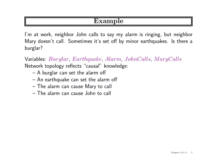
Example Im at work, neighbor John calls to say my alarm is ringing, but neighbor Mary doesnt call. Sometimes its set o ff by minor earthquakes. Is there a burglar? Variables: Burglar , Earthquake , Alarm , JohnCalls , MaryCalls Network
Example I’m at work, neighbor John calls to say my alarm is ringing, but neighbor Mary doesn’t call. Sometimes it’s set o ff by minor earthquakes. Is there a burglar? Variables: Burglar , Earthquake , Alarm , JohnCalls , MaryCalls Network topology reflects “causal” knowledge: – A burglar can set the alarm o ff – An earthquake can set the alarm o ff – The alarm can cause Mary to call – The alarm can cause John to call Chapter 14.1–3 5
Example contd. P(E) P(B) Burglary Earthquake .001 .002 B E P(A|B,E) T T .95 Alarm T F .94 F T .29 F F .001 A P(J|A) A P(M|A) T .90 JohnCalls .70 MaryCalls T F .05 .01 F Chapter 14.1–3 6
Compactness A CPT for Boolean X i with k Boolean parents has 2 k rows for the combinations of parent values B E A Each row requires one number p for X i = true (the number for X i = false is just 1 − p ) J M If each variable has no more than k parents, the complete network requires O ( n · 2 k ) numbers I.e., grows linearly with n , vs. O (2 n ) for the full joint distribution For burglary net, 1 + 1 + 4 + 2 + 2 = 10 numbers (vs. 2 5 − 1 = 31 ) Chapter 14.1–3 7
Global semantics Global semantics defines the full joint distribution B E as the product of the local conditional distributions: P ( x 1 , . . . , x n ) = Π n A i = 1 P ( x i | parents ( X i )) J M e.g., P ( j ∧ m ∧ a ∧ ¬ b ∧ ¬ e ) = Chapter 14.1–3 8
Global semantics “Global” semantics defines the full joint distribution B E as the product of the local conditional distributions: P ( x 1 , . . . , x n ) = Π n A i = 1 P ( x i | parents ( X i )) J M e.g., P ( j ∧ m ∧ a ∧ ¬ b ∧ ¬ e ) = P ( j | a ) P ( m | a ) P ( a |¬ b, ¬ e ) P ( ¬ b ) P ( ¬ e ) = 0 . 9 × 0 . 7 × 0 . 001 × 0 . 999 × 0 . 998 ≈ 0 . 00063 Chapter 14.1–3 9
Local semantics Local semantics: each node is conditionally independent of its nondescendants given its parents U 1 U m . . . X Z 1j Z nj Y Y n 1 . . . Theorem: Local semantics global semantics ⇔ Chapter 14.1–3 10
Markov blanket Each node is conditionally independent of all others given its Markov blanket: parents + children + children’s parents U 1 U m . . . X Z 1j Z nj Y n Y 1 . . . Chapter 14.1–3 11
Constructing Bayesian networks Need a method such that a series of locally testable assertions of conditional independence guarantees the required global semantics 1. Choose an ordering of variables X 1 , . . . , X n 2. For i = 1 to n add X i to the network select parents from X 1 , . . . , X i − 1 such that P ( X i | Parents ( X i )) = P ( X i | X 1 , . . . , X i − 1 ) This choice of parents guarantees the global semantics: P ( X 1 , . . . , X n ) = Π n i = 1 P ( X i | X 1 , . . . , X i − 1 ) (chain rule) = Π n i = 1 P ( X i | Parents ( X i )) (by construction) Chapter 14.1–3 12
Example Suppose we choose the ordering M , J , A , B , E MaryCalls JohnCalls P ( J | M ) = P ( J ) ? Chapter 14.1–3 13
Example Suppose we choose the ordering M , J , A , B , E MaryCalls JohnCalls Alarm P ( J | M ) = P ( J ) ? No P ( A | J, M ) = P ( A | J ) ? P ( A | J, M ) = P ( A ) ? Chapter 14.1–3 14
Example Suppose we choose the ordering M , J , A , B , E MaryCalls JohnCalls Alarm Burglary P ( J | M ) = P ( J ) ? No P ( A | J, M ) = P ( A | J ) ? P ( A | J, M ) = P ( A ) ? No P ( B | A, J, M ) = P ( B | A ) ? P ( B | A, J, M ) = P ( B ) ? Chapter 14.1–3 15
Example Suppose we choose the ordering M , J , A , B , E MaryCalls JohnCalls Alarm Burglary Earthquake P ( J | M ) = P ( J ) ? No P ( A | J, M ) = P ( A | J ) ? P ( A | J, M ) = P ( A ) ? No P ( B | A, J, M ) = P ( B | A ) ? Yes P ( B | A, J, M ) = P ( B ) ? No P ( E | B, A, J, M ) = P ( E | A ) ? P ( E | B, A, J, M ) = P ( E | A, B ) ? Chapter 14.1–3 16
Example Suppose we choose the ordering M , J , A , B , E MaryCalls JohnCalls Alarm Burglary Earthquake P ( J | M ) = P ( J ) ? No P ( A | J, M ) = P ( A | J ) ? P ( A | J, M ) = P ( A ) ? No P ( B | A, J, M ) = P ( B | A ) ? Yes P ( B | A, J, M ) = P ( B ) ? No P ( E | B, A, J, M ) = P ( E | A ) ? No P ( E | B, A, J, M ) = P ( E | A, B ) ? Yes Chapter 14.1–3 17
Example contd. MaryCalls JohnCalls Alarm Burglary Earthquake Deciding conditional independence is hard in noncausal directions (Causal models and conditional independence seem hardwired for humans!) Assessing conditional probabilities is hard in noncausal directions Network is less compact: 1 + 2 + 4 + 2 + 4 = 13 numbers needed Chapter 14.1–3 18
Compact conditional distributions CPT grows exponentially with number of parents CPT becomes infinite with continuous-valued parent or child Solution: canonical distributions that are defined compactly Deterministic nodes are the simplest case: X = f ( Parents ( X )) for some function f E.g., Boolean functions NorthAmerican ⇔ Canadian ∨ US ∨ Mexican E.g., numerical relationships among continuous variables ∂ Level = inflow + precipitation - outflow - evaporation ∂ t Chapter 14.1–3 21
Compact conditional distributions contd. Noisy-OR distributions model multiple noninteracting causes 1) Parents U 1 . . . U k include all causes (can add leak node) 2) Independent failure probability q i for each cause alone ⇒ P ( X | U 1 . . . U j , ¬ U j +1 . . . ¬ U k ) = 1 − Π j i = 1 q i Cold Flu Malaria P ( Fever ) P ( ¬ Fever ) F F F 1 . 0 0.0 F F T 0 . 9 0.1 F T F 0 . 8 0.2 F T T 0 . 98 0 . 02 = 0 . 2 × 0 . 1 T F F 0 . 4 0.6 T F T 0 . 94 0 . 06 = 0 . 6 × 0 . 1 T T F 0 . 88 0 . 12 = 0 . 6 × 0 . 2 T T T 0 . 988 0 . 012 = 0 . 6 × 0 . 2 × 0 . 1 Number of parameters linear in number of parents Chapter 14.1–3 22
Hybrid (discrete+continuous) networks Discrete ( Subsidy ? and Buys ? ); continuous ( Harvest and Cost ) Subsidy? Harvest Cost Buys? Option 1: discretization—possibly large errors, large CPTs Option 2: finitely parameterized canonical families 1) Continuous variable, discrete+continuous parents (e.g., Cost ) 2) Discrete variable, continuous parents (e.g., Buys ? ) Chapter 14.1–3 23
Continuous child variables Need one conditional density function for child variable given continuous parents, for each possible assignment to discrete parents Most common is the linear Gaussian model, e.g.,: P ( Cost = c | Harvest = h, Subsidy ? = true ) = N ( a t h + b t , σ t )( c ) 2 1 − 1 c − ( a t h + b t ) = 2 π exp √ 2 σ t σ t Mean Cost varies linearly with Harvest , variance is fixed Linear variation is unreasonable over the full range but works OK if the likely range of Harvest is narrow Chapter 14.1–3 24
Continuous child variables P(Cost|Harvest,Subsidy?=true) 0.35 0.3 0.25 0.2 0.15 0.1 0.05 0 10 0 5 Harvest 5 Cost 10 0 All-continuous network with LG distributions full joint distribution is a multivariate Gaussian ⇒ Discrete+continuous LG network is a conditional Gaussian network i.e., a multivariate Gaussian over all continuous variables for each combination of discrete variable values Chapter 14.1–3 25
Discrete variable w/ continuous parents Probability of Buys ? given Cost should be a “soft” threshold: 1 0.8 P(Buys?=false|Cost=c) 0.6 0.4 0.2 0 0 2 4 6 8 10 12 Cost c Probit distribution uses integral of Gaussian: � x Φ ( x ) = −∞ N (0 , 1)( x ) dx P ( Buys ? = true | Cost = c ) = Φ (( − c + µ ) / σ ) Chapter 14.1–3 26
Why the probit? 1. It’s sort of the right shape 2. Can view as hard threshold whose location is subject to noise Cost Cost Noise Buys? Chapter 14.1–3 27
Discrete variable contd. Sigmoid (or logit) distribution also used in neural networks: 1 P ( Buys ? = true | Cost = c ) = 1 + exp ( − 2 − c + µ σ ) Sigmoid has similar shape to probit but much longer tails: 1 0.9 0.8 P(Buys?=false|Cost=c) 0.7 0.6 0.5 0.4 0.3 0.2 0.1 0 0 2 4 6 8 10 12 Cost c Chapter 14.1–3 28
Summary Bayes nets provide a natural representation for (causally induced) conditional independence Topology + CPTs = compact representation of joint distribution Generally easy for (non)experts to construct Canonical distributions (e.g., noisy-OR) = compact representation of CPTs Continuous variables ⇒ parameterized distributions (e.g., linear Gaussian) Chapter 14.1–3 29
Inference tasks Simple queries: compute posterior marginal P ( X i | E = e ) e.g., P ( NoGas | Gauge = empty, Lights = on, Starts = false ) Conjunctive queries: P ( X i , X j | E = e ) = P ( X i | E = e ) P ( X j | X i , E = e ) Optimal decisions: decision networks include utility information; probabilistic inference required for P ( outcome | action, evidence ) Value of information: which evidence to seek next? Sensitivity analysis: which probability values are most critical? Explanation: why do I need a new starter motor? Chapter 14.4–5 3
Inference by enumeration Slightly intelligent way to sum out variables from the joint without actually constructing its explicit representation Simple query on the burglary network: B E P ( B | j, m ) = P ( B, j, m ) /P ( j, m ) A = α P ( B, j, m ) = α Σ e Σ a P ( B, e, a, j, m ) J M Rewrite full joint entries using product of CPT entries: P ( B | j, m ) = α Σ e Σ a P ( B ) P ( e ) P ( a | B, e ) P ( j | a ) P ( m | a ) = α P ( B ) Σ e P ( e ) Σ a P ( a | B, e ) P ( j | a ) P ( m | a ) Recursive depth-first enumeration: O ( n ) space, O ( d n ) time Chapter 14.4–5 4
Recommend
More recommend
Explore More Topics
Stay informed with curated content and fresh updates.

