Introduction to Accelerated Molecular Dynamics Methods Danny Perez - PowerPoint PPT Presentation

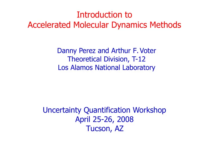
Introduction to Accelerated Molecular Dynamics Methods Danny Perez and Arthur F. Voter Theoretical Division, T-12 Los Alamos National Laboratory Uncertainty Quantification Workshop April 25-26, 2008 Tucson, AZ

Acknowledgments Blas P. Uberuaga (LANL, MST-8) Francesco Montalenti (U. Milano-Bicocca) Graeme Henkelman (U. Texas at Austin) James A. Sprague (NRL) Mads Sorensen (Novo Nordisk A/S, Copenhagen) Sriram Swaminarayan (LANL, MST-8) Steve Stuart (Clemson) Roger Smith (U. Loughborough) Robin Grimes (Imperial College) Kurt Sickafus (LANL, MST-8) Jacques Amar (U. Toledo) Yunsic Shim (U. Toledo) Yuri Mishin (George Mason U.) Soo Young Kim (LANL postdoc, T-12) Abhijit Chatterjee (LANL postdoc, T-12) DOE Office of Basic Energy Sciences LDRD (LANL Internal) SCIDAC (DOE)

Outline • The molecular dynamics (MD) timescale problem • Infrequent-event systems • Transition State Theory • Accelerated molecular dynamics methods – Hyperdynamics – Parallel-replica dynamics – Temperature accelerated dynamics (TAD) • Ongoing challenges and recent advances • Conclusion

The MD time-scale problem For many systems, we need to simulate with full atomistic detail. Molecular dynamics (MD) (the integration of the atomistic equations of motion) can only reach nanoseconds to microseconds due to the stiffness of the equations of motion (timestep is limited to fs). Processes we want to study often take much longer: - vapor-deposited film growth (s) - STM/AFM surface manipulation, nanoindentation (ms - s) - bulk and surface diffusion processes - radiation damage annealing (ns, µ s, ms, s, …, years) - protein folding ( µ s - s) Such slowly evolving systems share a common feature: their long-time dynamics consists of infrequent jumps between different states (i.e., activated processes). The problem is that these systems are way too complex to map out completely. We thus cannot use Kinetic Monte Carlo to generate long-time trajectories.

Infrequent Event System Indeed, the system vibrates in one of the 3N dimensional basins many times before finding an escape path. The trajectory finds an appropriate way out (i.e., proportional to the rate constant) without knowing about any of the escape paths except the one it first sees. Can we exploit this?

Transition State Theory (TST) Marcelin (1915) Eyring, Wigner,… TST escape rate = equilibrium flux through dividing surface at x=q TST = 〈 x − q ∣ ˙ x ∣〉 A = Z q / Z A (exact flux) k A  B (harmonic approx.) − Δ E / k B T HTST = υ 0 e k A  B - classically exact rate if no recrossings or correlated events - no dynamics required - excellent approximation for materials diffusion - entails an exponential distribution of escape times

Accelerated molecular dynamics (AMD) concept Let the trajectory, which is smarter than we are, find an appropriate way out of each state. The key is to coax it into doing so more quickly, using statistical mechanical concepts (primarily transition state theory). With these AMD methods, we can follow a system from state to state, reaching time scales that we can’t achieve with molecular dynamics. However, we have to sacrifice the short time dynamics to do so. AMD methods are not sampling methods as they generate a single long state- to-state trajectory at the time. Often, even just one of these long trajectories can reveal key system behavior. If desired, we can go back through the trajectory to determine rates and properties in more detail, using conventional methods, and/or we can run more long trajectories to gather statistics.

Accelerated Molecular Dynamics Methods Hyperdynamics (1997) • Design bias potential that fills basins. • MD on biased surface evolves correctly from state to state. • Accelerated time is statistical quantity. Parallel Replica Dynamics (1998) • Parallelizes time. • Very general -- any exponential process. • Gives exact dynamics. • Boost requires multiple processors Temperature Accelerated Dynamics (2000) • Raise temperature of MD in this basin. • Intercept and block every attempted escape. • Accept event that would have occurred first at the low temperature. • More approximate; good boost.

Characteristics of the AMD methods All three methods can give very large boost factors when events are very ● infrequent ps ns µ s ms s • Hyperdynamics – requires designing a valid and effective bias potential – assumes TST holds (no recrossings) – no need to detect transitions • Parallel Replica Dynamics – requires M processors for boost of M – most general, most accurate – can treat entropic bottlenecks • Temperature Accelerated Dynamics – most approximations, but still fairly accurate – assumes harmonic transition state theory

Parallel-Replica Parallel-Replica Dynamics Dynamics

Parallel Replica Dynamics Concept: Follow many replicas of the system on a parallel computer to parallelizes time evolution Assumptions: - exponential distribution of first-escape times p  t  = k exp − k t  p(t) Must know: t - how to detect transitions - correlation time AFV, Phys. Rev. B, 57, R13985 (1998)

Parallel Replica Dynamics Procedure Replicate entire system on each of M processors.

Parallel Replica Dynamics Procedure Randomize momenta independently on each processor.

Parallel Replica Dynamics Procedure Run MD for short time ( τ dephase ) to dephase the replicas.

Parallel Replica Dynamics Procedure Start clock and run thermostatted MD on each processor. Watch for transition…

Parallel Replica Dynamics Procedure Stop all trajectories when first transition occurs on any processor.

Parallel Replica Dynamics Procedure Sum the trajectory times over all M processors. Advance simulation clock by this t sum

Parallel Replica Dynamics Procedure On the processor where a transition occurred, continue trajectory for a time τ corr to allow correlated dynamical events.

Parallel Replica Dynamics Procedure Advance simulation clock by τ corr .

Parallel Replica Dynamics Procedure Replicate the new state and begin procedure again.

Long time annealing of 20 vacancy void in Cu • EAM Copper • Parallel-replica simulation of 20-vacancy void annealing at T=400 K - 20 vacancies is one too many for “perfect” void Total simulation is 7.82 µ s • At 1.69 µ s, void transforms to SFT • • Equivalent single processor time: 1.3 years • Very complex transition pathway Red atoms=vacancies Completely new transformation Blue atoms=interstitials pathway for the formation of Bulk atoms not shown stacking fault tetrahdera (SFT) Uberuaga, Hoagland, Voter, Valone, PRL 99 , 135501 (2007)

Transformation pathway for 20 vacancy void • Full path for transformation to SFT calculated with NEB • Initial barrier is >2 eV • Vineyard prefactor for first step is 2x10 36 Hz ! • Driven by entropy increase as extra volume is made available to system as void collapses Uberuaga, Hoagland, Voter, Valone, PRL 99 , 135501 (2007)

Summary: Parallel Replica Dynamics The summed time (t sum ) obeys the correct exponential distribution, and the system escapes to an appropriate state. State-to-state dynamics are thus correct; τ corr stage even releases the TST assumption [AFV, Phys. Rev. B, 57, R13985 (1998)]. Maximal boost is equal to M Good parallel efficiency if τ rxn / M >> τ dephase + τ corr Applicable to any system with exponential first-event statistics

Hyperdynamics Hyperdynamics

Hyperdynamics Concept: Fill the basins with a bias potential to increase the rate of escape and renormalize the time accordingly. Assumptions: - transition state theory (no recrossings) V+ Δ V Procedure: V - design bias potential Δ V which is zero at all dividing surfaces so as not to bias rates along different pathways. - run thermostatted trajectory on the biased surface (V+ Δ V) - accumulate hypertime as t hyper = Σ Δ t MD exp[ Δ V(R(t))/k B T] Result: - state-to-state sequence correct - time converges on correct value in long-time limit (vanishing relative error) AFV, J. Chem. Phys. 106, 4665 (1997)

The hypertime clock System coordinate MD clock hypertime clock Δ t MD

The hypertime clock System coordinate MD clock hypertime clock Δ t MD Δ t hyper

The hypertime clock System coordinate MD clock hypertime clock Δ t MD Δ t hyper Boost = hypertime/(MD clock time)

Hyperdynamics Key challenge is designing a bias potential that meets the requirements of the derivation and is computationally efficient. This is very difficult since we do not have any a priori information about neighboring states nor about the dividing surfaces in between them. Futher, we have to work in very high dimension. A few forms have been proposed and tested. Still a subject of ongoing research… We recently proposed a self-learning version of the Bond-Boost potential of Miron and Fichthorn that automatically adapts to the system at hand, thus requiring no a priori parametrization. For discussion, see Voter, Montalenti, and Germann, Ann. Rev. Mater. Res. 32, 321 (2002)