Introduction Suppose that an economic relationship can be - PDF document
Lecture 2: Marginal Functions, Average Functions, Elasticity, the Marginal Principle, and Constrained Optimization The marginal or derivative function and optimization-basic principles The average function Elasticity Basic
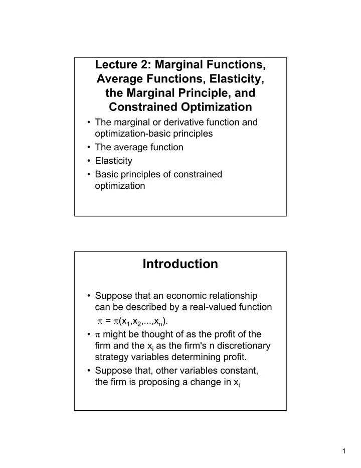
Lecture 2: Marginal Functions, Average Functions, Elasticity, the Marginal Principle, and Constrained Optimization • The marginal or derivative function and optimization-basic principles • The average function • Elasticity • Basic principles of constrained optimization Introduction • Suppose that an economic relationship can be described by a real-valued function = (x 1 ,x 2 ,...,x n ). • might be thought of as the profit of the firm and the x i as the firm's n discretionary strategy variables determining profit. • Suppose that, other variables constant, the firm is proposing a change in x i 1
Introduction • Redefine x i as x and write (x), where x now denotes the single discretionary variable x i . The marginal or derivative function • Relative to some given level of x, we might be interested in the effect on of changing x by some amount x ( x denotes a change in x). • If x takes on the two values x' and x'', then x = (x'' - x'). We could form the difference quotient x = ( ' x x ) ( ') x (1) . x 2
Marginal function • In the following figure, we illustrate / x by the slope of the line segment AB. slope = '(x') B (x'+ x) A slope = / x (x') x' x'' = x'+ x x Figure 1 Marginal function • If we take the limit of / x as x 0, that is, / x = '(x'), lim x 0 then we obtain the marginal or derivative function of . • Geometrically, the value of the derivative function is given by the slope of the tangent to the graph of at the point A (i.e., the point (x', (x')) ). 3
Illustrations: Total and Marginal ' ' x x Figure 2 Figure 3 Discussion of Figures 2,3 • In Figures 2,3 we show two total functions and their respective marginal functions. • Figure 2 depicts a total function having a maximum and Figure 3 depicts a total function having a minimum. • Note that at maximum or a minimum point, the total function flattens out, or its marginal function goes to zero. In economics, we refer to this as the marginal principle. 4
Marginal Principle • The marginal principal states that the value of the marginal function is zero at any extremum (maximum or minimum) of the total function. • This principal can be extended to state that if at a point x we have that '(x) > 0, then in a neighborhood of x, we should raise x if we are interested in maximizing and lower x if we are interested in minimizing . Marginal Principal • This principle assumes that the total function is hill shaped in the case of a maximum and valley shaped in the case of a minimum. • There are second order conditions which suffice to validate a zero marginal point as a maximum or a minimum. 5
Second order conditions • For a maximum, it would be true that in a neighborhood of the extremum, we have that the marginal function is decreasing or downward sloping. • For a minimum, the opposite would be true. Second order conditions • For a maximum, it would be true that in a neighborhood of the extremum, we have that the marginal function is decreasing or downward sloping. • For a minimum, the opposite would be true. 6
Example • Let (x) = R(x) - C(x), where R is a revenue function and C is a cost function. The variable x might be thought of as the level of the firm's output. Suppose that a maximum of the firm's profit occurs at the output level x o . Then we have that '(x o ) = R'(x o ) - C'(x o ) = 0, or that • R'(x o ) = C'(x o ). Example • At a profit maximum, marginal revenue is equal to marginal cost. • Using the marginal principle, the firm should raise output when marginal revenue is greater than marginal cost, and it should lower output when marginal revenue is less than marginal cost. 7
Many choice variables • If the firm's objective function has n strategy variables x = (x 1 ,...,x n ), then the marginal function of the i th strategy variable is denoted as i • We define i in the same way that ' was defined above with the stipulation that all other choice variables are held constant when we consider the marginal function of the i th . Many choice variables • For example if we were interested in 1 ' ' ' ' ' / x 1 = ( x x , x ,..., x ) ( x ,..., x ) 1 1 2 n 1 n (2) . x 1 • Taking the limit of this quotient as x 1 tends to zero we obtain the marginal function 1 . The other i are defined in an analogous fashion. 8
Marginal principle: many choice variables • At a maximum or at a minimum of the total function, all of the values of the marginal functions go to zero. • If x o = (x 1 o ,..., x n o ) is the extremum, then we would have that i (x 1 o ,..., x n o ) = 0. for all i. Marginal principle: many choice variables • If we were searching for a maximum, then we would raise any strategy variable whose marginal function has a positive value at a point, and we would lower a strategy variable whose marginal function has a negative value at a point. • The reverse recommendations would be made if we were interested in finding a minimum. 9
The average function • Given the total function (x), the corresponding average function is defined by ( ) x , for x 0. (3) x Illustration of average function • Geometrically, at any x o , the average function at x o is given by the slope of the line segment joining zero and the point (x o , (x o )). (x o ) slope = (x o )/x o 0 x o x Figure 4 10
Example C (x) x o x C (x)/x x o x F igu re 5 Discussion of example • Let C = C(x) denote a firm's cost function and let x be the firm's level of output. • In the lower diagram, we show C(x)/x, termed average cost. • Average cost has two regions. In the initial region, average cost is declining as output is increased, and, in the second region, the opposite is true. 11
Elasticity • The notion of elasticity is used in many business applications where the objective is to gauge the responsiveness of one variable to a change in another variable. • A firm to wants to know how a rival's price change might impact the quantity demanded of their product. • Alternatively, the same firm might want to quantify the impact on quantity demanded of their product of a change in the price of their product or a change in advertising outlay for that product . Elasticity • Elasticity measures the impact of such changes by taking the percentage change in a dependent variable induced by some percentage change in an independent variable. / / x (4) = (m arginal function) / (average function). x x / / x 12
Measurement • If one knows through empirical estimation, then the marginal function can be used for the difference quotient / x. • In this case, the elasticity is called a point elasticity . • In some cases, the function is not known and only observations of x and are available. Measurement • If we have at least two observations of (x, ), then we can compute a different notion of elasticity called the arc elasticity . '' ' x a ( ) (5) a . ( '' x x ') average observations are denoted x a and a 13
Example #1 • Let the function Q = 12 - 4p = Q(p) describe a demand relationship, where p is price and Q is quantity. Given that this function is linear, we have that Q'(p) = Q/ p = - 4. The point elasticity at the price level p = $1 is given by Q p p '( ) 4 1 ( ) 4 1 2 . Q 12 4 1 ( ) 8 Example #2 • We observe that when p = $2, Q = 10. Further when p = $4, we have that Q = 6. Compute the arc elasticity of demand for these observations. Q / p [( 6 10 ) / ( 4 2 )] 2 3 ( ) 3 . a a Q / p 8 3 / 8 4 14
Constrained Optimization: Basic Principles • In many business problems, we are confronted with a feasibility constraint which limits our ability to choose values of our strategy variables. • As an example, consider the problem of maximizing output flow given a limited budget to purchase the inputs used to produce output. • Alternatively, a manager may be asked to achieve an output target with a cost minimal choice of inputs. Constrained Optimization • A firm has just two strategy variables, x 1 , x 2 . • We assume that the two strategy variables generate an output variable q which the firm sells. The relationship between the two variables and output is given by the multi-variable function (6) q = f(x 1 ,x 2 ). 15
Recommend
More recommend
Explore More Topics
Stay informed with curated content and fresh updates.


