Introduction Thermodynamics: phenomenological description of - PDF document

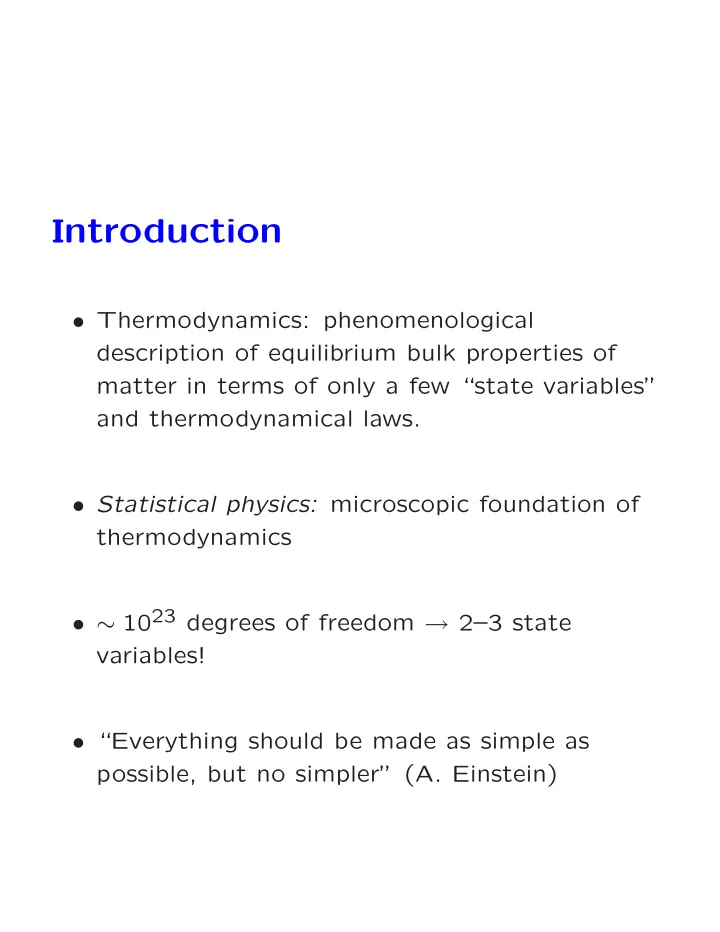
Introduction • Thermodynamics: phenomenological description of equilibrium bulk properties of matter in terms of only a few “state variables” and thermodynamical laws. • Statistical physics: microscopic foundation of thermodynamics • ∼ 10 23 degrees of freedom → 2–3 state variables! • “Everything should be made as simple as possible, but no simpler” (A. Einstein)

Summary of contents: • Review of thermodynamics • Thermodynamical potentials • Phase space and probability • Quantum mechanical ensembles • Equilibrium ensembles • Ideal fluids • Bosonic systems • Fermionic systems • Interacting systems • Phase transitions and critical phenomena

1. Foundations of thermodynamics 1.1. Fundamental thermodynamical concepts System : macroscopic entity under consideration. Environment : world outside of the system (infinite). Open system : can exchange matter and heat with the environment. Closed system : can exchange heat with the environment while keeping the number of particles fixed. Isolated system : can exchange neither matter nor heat with the environment. Can (possibly) still do work by e.g. expanding.

Thermodynamical equilibrium: • No macroscopic changes. • Uniquely described by (a few) external variables of state. • System forgets its past: no memory effects, no hysteresis. • Often the term global equilibrium is used, as opposed to local equilibrium, which is not full equilibrium at all (next page)!

Nonequilibrium: • Generally much more complicated than equilibrium state. • Simplest case: isolated systems each in an equilibrium state. • In a local thermodynamical equilibrium small regions are locally in equilibrium, but neighbour regions in different equilibria ⇒ particles, heat etc. will flow. Example: fluid (water) with non-homogeneous temperature. • Stronger nonequilibrium systems usually relax to a local equilibrium.

Degrees of freedom (d.o.f.) is the number of quantities needed for the exact description of the microscopic state. Example: classical ideal gas with N particles: 3 N coordinates ( x, y, z ), 3 N momenta ( p x , p y , p z ). State variables are parameters characterizing the macroscopic thermodynamical state. These are all extensive or intensive : Extensive variable: change value when the size (spatial volume and the number of degrees of freedom) is changed: volume V , particle number N , internal energy U , � d 3 r M . entropy S , total magnetic moment Intensive variable: independent of the size of the system, and can be determined for every semimicroscopical volume element: e.g. temperature T , pressure p , chemical potential µ , magnetic field H , ratios of extensive variables like ρ = N/V , s = S/N, . . . .

Conjugated variables: A and B appear in pairs in expressions for the differential of the energy (or more generally, some state variable), i.e. in forms ± A dB or ± B dA ; one is always extensive and the other intensive. Example: pressure p and volume V ; change in internal energy U when V is changed (adiabatically, at constant S ) is dU = − pdV .

Process is a change in the state. Reversible process: advances via states infinitesimally close to equilibrium, quasistatically (“slow process”). The direction of a reversible process can be reversed, obtaining the initial state (for system + environment!) Isothermal process : T constant. Isobaric process : p constant. Isochoric process : V constant. Isentropic or adiabatic process : S constant. Irreversible process is a sudden or spontaneous change during which the system is far from equilibrium. In the intermediate steps global state variables ( p , T , . . . ) are usually not well defined. Cyclic process consists of cycles which take the system every time to its initial state.

1.2. State variables and exact differentials Let us suppose that, for example, the state of the system can be uniquely described by state variables T , V ja N . Other state variables are then their unique functions: p = p ( T, V, N ) U = U ( T, V, N ) S = S ( T, V, N ) . . . By applying differential calculus, the differential of p , for example, is � ∂p � ∂p � ∂p � � � dp = dT + dV + dN ∂T ∂V ∂N V,N T,N T,V . . .

� � � � The differentials of state variables, dp , dT , dV , . . . , are exact differentials . These have the following properties (A) Their total change evaluated over a closed path vanishes: � � � � � 1 → 2 dp = 1 → 2 dU = · · · = 0 . (B) The total change of an exact differential is independent on the path of integration: � � b dU = 0 , a dU − so that we can write � 2 U (2) = U (1) + 1 dU

Exact differentials Let us denote by ¯ dF a differential which is not necessarily exact (i.e. integrals can depend on the path). Assuming it depends on 2 variables x, y , the differential dF = F 1 ( x, y ) dx + F 2 ( x, y ) dy ¯ is exact differential if ∂F 1 ∂y = ∂F 2 ∂x . Then ∃ F ( x, y ) so that F 1 ( x, y ) = ∂F ( x,y ) and ∂x F 2 ( x, y ) = ∂F ( x,y ) and ∂y � 2 dF = F (2) − F (1) 1 ¯ is independent on the path, and integrable. In this case ( x, F 1 ) and ( y, F 2 ) are pairs of conjugated variables with respect to F . Examples: are the following differentials exact? dF = y dx + x dy ¯ dF = x dx + x dy ¯

All physical state variables are exact differentials! This will enable us to derive various identities between state variables. Integrating factor If ¯ dF = F 1 dx + F 2 dy is not exact, there exists an integrating factor λ ( x, y ) so that in the neighbourhood of the point ( x, y ) λ ¯ dF = λF 1 dx + λF 2 dy = d f is an exact differential. λ and f are state variables. Example: find λ for the differential dF = x dx + x dy . ¯

Legendre transformations Legendre transformations can be used to make changes in the set of the indepependent state variables. For example, let us look at the function f ( x, y ) of two variables. We denote z = f y = ∂f ( x, y ) ∂y and define the function g = f − yf y = f − yz. (Note: z, y is a congjugated pair with respect to f !) Now dg = d f − y dz − z dy = f x dx + f y dy − y dz − z dy = f x dx − y dz. Thus we can take x and z as independent variables of the function g , i.e. g = g ( x, z ). Obviously y = − ∂g ( x, z ) . ∂z Corresponding to the Legendre transformation f → g there is the inverse transformation g → f f = g − zg z = g + yz.

Often needed identities Let F = F ( x, y ), x = x ( y, z ), y = y ( x, z ) and z = z ( x, y ). If we want to give F in terms of ( x, z ), we can write F ( x, y ) = F ( x, y ( x, z )) . Applying differential rules we obtain identities � � � ∂F � ∂F ∂F � ∂y � � � = + ∂x ∂x ∂y ∂x z y z x � � � ∂F ∂F � ∂y � � = ∂z ∂y ∂z x x x One can show that � � ∂x 1 = � ∂y � ∂y z ∂x z � � ∂x � ∂y � ∂z � � = − 1 ∂y ∂z ∂x x y z and � ∂F � � � ∂x ∂y z = . � ∂F � ∂y z ∂x z

1.3. Equations of state Encodes (some of the) physical properties of the equilibrium system. Usually these relate “mechanical” readily observable variables, like p , T , N , V ; not “internal” variables like S , internal energy U etc. A typical example: pressure of some gas as a function of T and density ρ . Some examples: Classical ideal gas pV = Nk B T where N = number of molecules T = absolute temperature k B = 1 . 3807 · 10 − 23 J/K = Boltzmann constant. Chemists use often the form pV = nRT = N/N 0 = number of moles n R = k B N 0 = 8 . 315J/K mol = gas constant 6 . 0221 · 10 23 = Avogadro’s number . N 0 =

If the gas is composed of m different species of molecules the equation of state is still pV = Nk B T, where now m � N = N i i =1 and � p = p i = N i k B T/V, p i , i where p i is the partial pressure of the i :th component Virial expansion of real gases When the interactions between gas molecules are taken into account, the ideal gas law receives corrections which are suppressed by powers of density ρ = N/V : � � ρ + ρ 2 B 2 ( T ) + ρ 3 B 3 ( T ) + · · · p = k B T Here B n is the n :th virial coefficient .

Van der Waals equation The molecules of real gases interact • repulsively at short distances; every particle needs at least the volume b ⇒ V > ∼ Nb . • attractively (potential ∼ ( r/r 0 ) 6 ) at large distances due to the induced dipole momenta. The pressure decreases when two particles are separated by the attraction distance. The probability of this is ∝ ( N/V ) 2 . We improve the ideal gas state equation p ′ V ′ = Nk B T so that V ′ = V − Nb p ′ − aρ 2 = true pressure . p = then ( p + aρ 2 )( V − Nb ) = Nk B T.

Solid substances The thermal expansion coefficient α p = 1 � ∂V � V ∂T p,N and the isothermal compressibility � � κ T = − 1 ∂V V ∂p T,N of solid materials are very small, so the Taylor series V = V 0 (1 + α p T − κ T p ) is a good approximation. Typically 10 − 10 / Pa κ T ≈ 10 − 4 / K . α p ≈

Stretched wire Tension [N/m 2 ] σ = E ( T )( L − L 0 ) /L 0 , where L 0 is the length of the wire when σ = 0 and E ( T ) is the temperature dependent elasticity coefficient. Surface tension � n 1 − t � = σ σ 0 t ′ temperature ◦ C t = t ′ and n experimental constants , 1 < ∼ n < ∼ 2 surface tension when t = 0 ◦ C . = σ 0